A Bayesian Model for Estimating Long Tailed Excess of Loss Reinsurance Loss Costs

undefined

1. INTRODUCTION

Cedent claim datasets used in the pricing of excess of loss reinsurance are often limited in size. Individual claim data is provided for claims above a certain threshold and can produce sparse excess claim count triangles for long tailed lines. In some cases, excess triangles might not be available. A difficult problem faced by reinsurance pricing actuaries is how much credibility to assign cedent experience with limited excess claims and how to blend this data with industry excess loss development patterns and exposure rating methods.

We introduce a hierarchical Bayesian model which allows us to specify prior distributions and use Bayes’ Theorem to estimate posterior distributions based on the data. The model is programmed in R and Stan. The code, a sample dataset and case studies are provided so users can easily experiment for themselves. The foundation of this model is a standard Poisson-Pareto compound frequency severity distribution with gamma prior distributions. It includes a claim count emergence model that combines a Weibull distribution with gamma marginal priors. Codependence between the two Weibull parameters, which was found in our study, is described using a copula function. The model is used in practice for multiple long-tailed lines of business at a major reinsurance company. The next section describes practical applicabilities and benefits practitioners can enjoy.

The fundamental question on excess loss frequency is whether observing very few claims reported in an immature year is due to low ultimate frequency or slow development. Conversely, does a high observed claim count in an immature year imply high ultimate frequency or just quick development? The answer is that it could be an indication of either situation or a combination of both. Observed claim counts inform our view on the ultimate frequency and development pattern. How strong of an indicator the observed claim counts are depends on the relative uncertainty in the ultimate frequency compared to the uncertainty in the development pattern. The frequency model compares the observed claim counts to the joint probability of that observation under the uncertain ultimate frequency distribution and uncertain development pattern, allowing the two major assumptions, i.e., prior distributions, to be weighed against each other simultaneously.

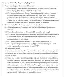
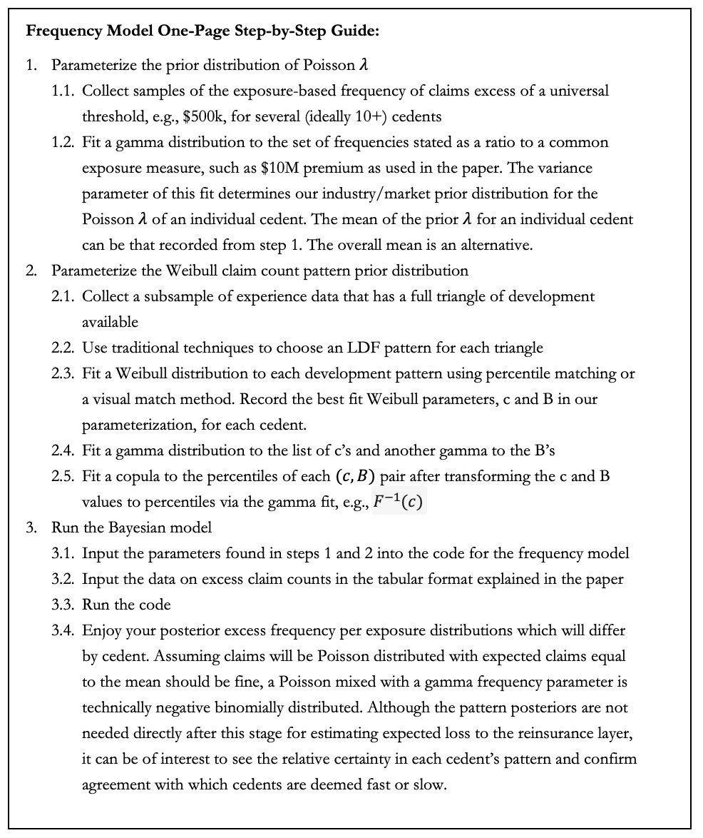
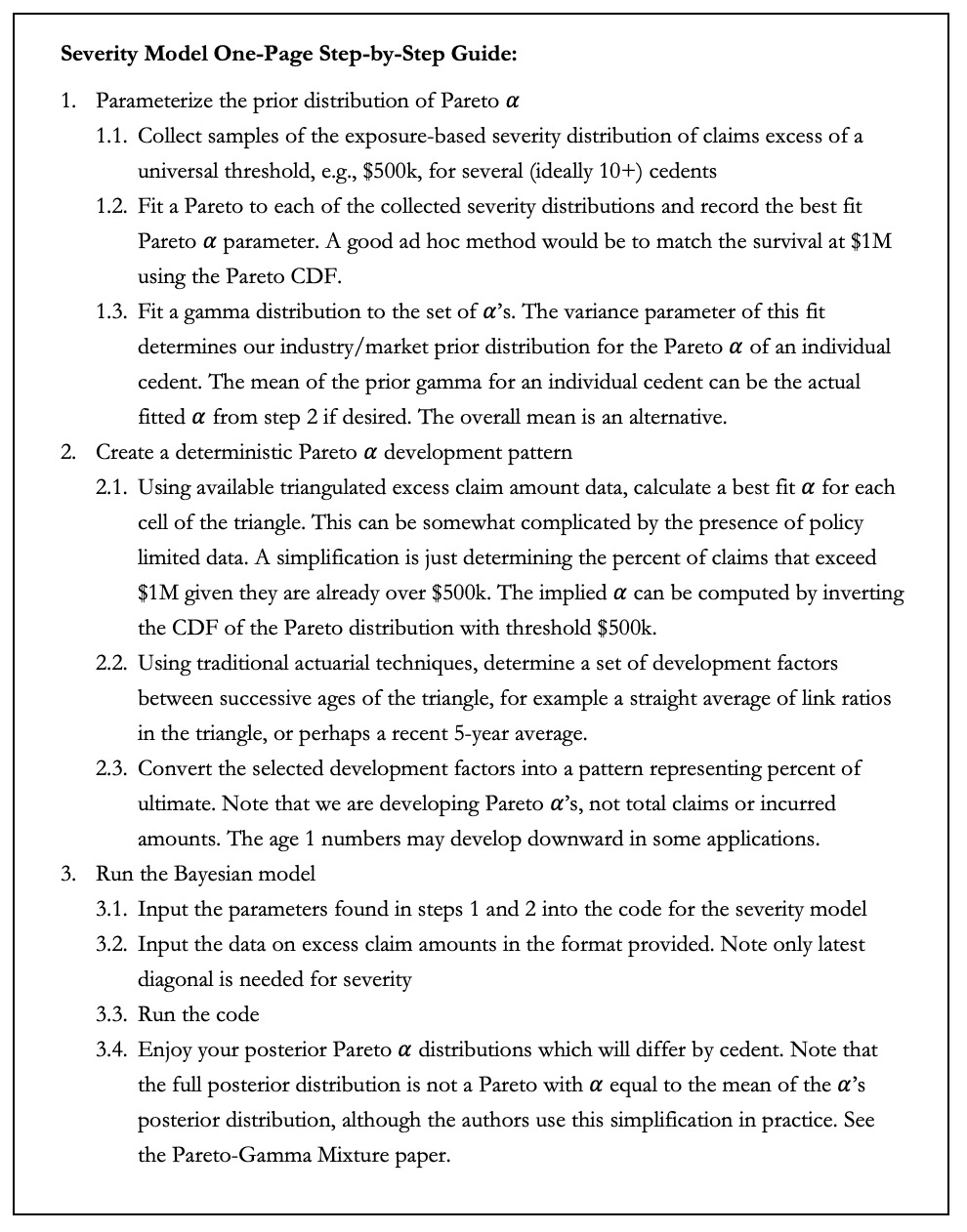
To complete the compound frequency severity distribution, we will also explain how to develop the Gamma-Pareto ultimate severity model. We will detail how our method addresses additional factors related to severity such as development, policy limit capping and loss adjustment expenses. Finally, we discuss comparisons to existing methods and Appendix A contains helpful one-page step-by-step guides to implementing the model in practice.

2. FREQUENCY MODEL

In this section we present a Bayesian frequency model for long-tailed, reinsurance excess of loss claim counts. A diagram of the frequency model is provided in Figure 1. Each component will be discussed at length in subsequent sections of this paper.

The quantity of interest in this model is the ultimate expected frequency per exposure, $\lambda$. However, we can only observe incremental claim counts in finite time intervals. A key concept is that claim counts are observed over a certain time period and the expected number of claims observed in that time period, given an expected ultimate frequency, is determined by the development pattern. The Poisson formula in the observation level of the diagram is the part of the model that connects the observed claim counts with the prior distributions of the development pattern and the ultimate expected frequency in order to estimate posterior distributions. The relative certainty or uncertainty in each of the two company level components of the diagram, i.e., ultimate expected frequency and development pattern, are simultaneously weighed against each other to derive posterior distributions.

Note that CDF(t₂) – CDF(t₁) is the incremental expected percent of claims reported according to the Weibull development pattern assumption, where CDF refers to the cumulative distribution function. Also note that a hyperparameter in the context of a Bayesian hierarchical model is simply a parameter of a prior distribution in the model. Adding an additional “hyper” prefix simply moves us one level up the model hierarchy of parameters and prior distributions.

The following are several advantages of the frequency model that we feel are important motivations for investing your time and understanding. Each advantage considers development pattern uncertainty or aims for a more consistent and efficient application of assumptions across cedents. We hope it will be useful for readers to know that these are actual benefits the authors have seen from the use of this model in a live reinsurance renewal pricing process, not just theoretical benefits that could potentially materialize. The technical explanation of the model continues in the next section.

Development Pattern Uncertainty

1. The frequency model incorporates development pattern uncertainty on large loss frequency. A common subjective consideration in reinsurance is the development pattern of the cedent and its relation to an assumed default pattern. Usually, a large amount of data is required in traditional pricing techniques to use a cedent pattern instead of a default pattern. Having an uncertain Weibull development distribution with prior hyperparameters allows the cedent data to inform the pattern, i.e., update the posterior, to the extent it is credible.

2. Frequency and development are evaluated at the same time and the model weighs the relative uncertainty in both. Observed claim counts by year and development period are compared to a distribution of possible observed claim counts based on the prior distributions of ultimate frequency and the incremental percent of claims reported. The claim count data contains information about both the development pattern and the ultimate frequency, and the model attempts to extract and separate that information according to the prior distributions and Bayes’ Theorem.

3. Data used in the frequency model can be triangulated or in last diagonal form – i.e., a large loss listing as of a particular date. The model has a way of judging the amount of information contained in a triangle. It differentiates credibility between triangulated and non-triangulated data so that credibility assignment increases when a cedent triangle is available.

Consistency

1. Actuarial judgement is applied in specification of the prior, not in the individual loss selection for each cedent or final loss estimate where a subjective credibility is assigned to experience. When given those priors, every cedent is analyzed on the same basis and thus removes some subjectivity of experience rating and credibility selection. The method of implying credibility is applied consistently among all cedents. Two cedents with same mean and amount of data will get same posterior results. No judgement is used in the selection of credibility, leading to a more consistent blending of exposure rating and experience.

2. The model meaningfully and consistently incorporates cedent data with few historical losses and sparse development triangles, including being able to use and appropriately update prior distributions when zero claims are observed. Credibility implied by the model varies by “sparseness” of the data triangle.

Efficiency

1. R and Stan codes derive posterior ultimate excess frequencies simultaneously for multiple cedents. This approach allows for increased efficiencies in the reinsurance pricing process. Prior distribution parameters and company priors can be updated during times of the year when a reinsurer’s workload is slower and not as hectic.

2. Closed form posteriors are unnecessary for this model because everything is programmed using R and Stan. Formulas are nice in theory but in practice there is usually a danger that long formulas in papers have typos, and there is the possibility of translation error between a formula in a paper and recreating that formula in Excel or a programming language. Bayesian MCMC produces samples of the posterior from which all desired values can be estimated without having to deal with algebraic formulas.

2.1. The Observation Level of the Hierarchical Model

We assume observed claims are Poisson distributed. When we observe a claim count in a certain time period, we can then compare that number with the theoretical mean of the Poisson which is a function of both the Weibull distribution of the development pattern and the gamma distribution of the expected ultimate frequency as shown in Figure 1.

We use the following parameterization of the Poisson distribution:

$$p(k;\lambda) = \frac{\lambda^{k}e^{- \lambda}}{k!}$$

One might ask, why not just develop claims to ultimate using traditional techniques, and then treat those ultimate claim counts as observations of a Poisson distribution to more directly infer the ultimate frequency posterior? The answer is that this does not incorporate pattern uncertainty. A traditional development to ultimate will not capture the greater uncertainty (and weaker information relative to the prior) of the newer ages. We believe the model presented in this paper is a relatively direct way of incorporating pattern uncertainty into a large loss frequency analysis.

2.2. Data Organization and Model Inputs

Our study included 35 cedents providing primary General Liability coverage. The approach outlined in this paper can also be applied to other long-tailed lines of business such as Auto Liability or Workers’ Compensation. Our General Liability dataset contained more than 12,500 claims with 3,100 claims above $500,000. All companies had at least 10 accident years of information with some going back 20 years. There were 10 cedents with triangulated individual claims data and the remainder only provided claims along the last diagonal.

Reporting thresholds in the dataset were not consistent for each company. Less than a handful of cedents provided ground up claims. The other thresholds ranged from $50,000 to $500,000 with $500,000 being the most common. Therefore, our Bayesian model was constructed with threshold of $500,000.

Table 1 shows how to organize input data for the frequency model. Incremental claim counts are excess of a fixed threshold for all years and all companies. Columns obs_start and obs_end indicate starting and ending points of an observation age.

Notice that starting observation ages are equal to zero in every year for Company 1. This set up is used when only the last diagonal of data is received. Compare this to Company 2 where data for year 2010 is entered based on a claim count triangle. The input file, and the Bayesian frequency model, is structured to accommodate both triangulated and non-triangulated data.

Regarding the issue of loss trend, the model uses nominal data as input rather than trended data. Under “observed claim counts” in Figure 1, we show the application of a detrend factor. This is an excess frequency trend factor which includes ground up severity trend and the impact on excess frequency from ground up severity trend. Appendix B includes the frequency model Stan code. An assumed detrend factor of 10% is entered in the body of the code.

Since the ultimate expected frequency value refers to the prospective analysis year, we detrend the frequency to an expected amount for each prior accident year. Losses increase in severity over time which implies that the expected ultimate frequency at a fixed nominal threshold should be lower for each previous year as one goes back in time.^[1] There is no provision or allowance in this model for uncertainty in the trend, such as a prior distribution of annual trend amount, but it could be added relatively easily.

Input data assumes all premium and exposures are brought to current levels. Exposure trend and other premium related trends are accounted for by using onlevel exposure or onlevel premium as data input under the “Premium” column in Table 1. Premium is used in our example as a proxy for exposure, but the most accurate measure of frequency is number of claims per exposure base.

An important note on Company 2 is with regard to the obs_end value of 10.5 for year 2010. Section 2.4 will provide details on how the frequency model is able to handle data with partial year development. Company 2 demonstrates a common reinsurance scenario where a 12-month claim count development triangle is provided with a partial last diagonal – e.g., as of mid-year or June 30^th.

When working with triangulated data, incremental claim counts are used because there is correlation between cumulative claims at each age. Modeling cumulative claim counts requires additional parameterization of the correlation between ages which is an unnecessary complication. We work with the simpler assumption that given an ultimate frequency and Weibull development pattern the observed claim counts from disjoint time periods are independent.

2.3. Ultimate Expected Frequency and Parameterizing the Prior

Ultimate expected frequency in the reinsurance layer is the quantity of interest because it determines the reinsurance loss cost. However, it is unobservable. We can only make inferences based on a prior distribution and observed claim counts at finite ages. Ultimate frequency is defined in the model as ultimate expected claim counts excess of a threshold per unit of premium.

An ultimate frequency prior, denoted by $\widehat{\lambda}$, is established for each company in the portfolio. The authors of this paper derived priors using an exposure model, see (Clark 2014) page 27-31. However, other methods of determining an a priori are also acceptable. In our study containing 35 cedents, a gamma distribution was a reasonable fit to the set of ultimate expected frequencies indicated by the classical exposure model.

We use the following parameterization of the gamma distribution:

$$f(\lambda;\alpha,\beta) = \frac{\beta^{\alpha}}{Г(\alpha)}\lambda^{\alpha - 1}e^{- \beta\lambda}$$

The mean of a gamma distribution is α/β. Therefore, we have:

$$\lambda_{prior\_ co\lbrack i\rbrack}\ \sim\ Г(\beta*{\widehat{\lambda}}_{prior\_ co\lbrack i\rbrack},\ \beta)$$

A universal value for β is assumed. It represents the variability of each individual cedent’s actual frequency from the exposure model estimate, which may be based only on a few variables such as state and product mix without accounting for things specific to the cedent like risk selection or claims handling skill/philosophy/etc.

Theoretically there is a difference between the variability among each company’s exposure model frequency, versus the amount a cedent could differ from their own exposure model, but in the absence of a good way of measuring the latter, we use the former as a proxy.

2.4. Claim Count Development

A distribution of excess claim count development patterns is assumed in order to recognize that losses develop differently for each cedent, and that each cedent’s development pattern is uncertain. The frequency model responds in a proper way to the data based on the level of certainty represented by the prior distributions of the development pattern.

It is preferable to select an excess claim count development pattern from a family of continuous distributions over discrete distributions. This allows for data with partial year development to be used as inputs into the model. Reinsurance submission data is rarely received as of December 31^st. Continuous distributions have the flexibility to model latest diagonals at non-integer values such as 6 months or 18 months.

A Weibull distribution was found to fit excess development patterns reasonably well for a substantial number of cedents. We will use the following notation for a cumulative claim count pattern:

$$F(x) = 1 - {e}^{- (x/B)^{c}};x \geq 0$$

The scale parameter, B, controls the development pattern speed with higher values corresponding to a longer tail. The value of this parameter approximates the number of years until claims reach 63% development to ultimate. To see this, plugging in x=B produces the following cumulative development regardless of the value of c:

$$F(B) = 1 - \frac{1}{e}$$

Figure 3 provides the development pattern under a Weibull distribution for fixed c and varying values for B. Much faster development is observed for lower B values while higher scale parameter values substantially slow down the development pattern.

According to Figure 4, the shape parameter, c, also impacts the length of the tail. Lower values increase the tail length while higher values shorten the length assuming similar ranges of B. The distribution also becomes more S-shaped with an increasing c value.

2.5. Parameterizing the Weibull Development Prior

Not all cedents have a full triangle or enough data to estimate a complete development pattern. Our dataset included 10 companies with triangulated individual claims. Of those companies, 8 had enough data with which to estimate a development pattern. This subset of cedents is used to parameterize the development pattern prior distributions. A Weibull distribution is assumed to describe the cumulative excess development pattern for each cedent with sufficient triangulated data. Judgement needs to be used as it typically is in selecting LDFs and the tail factor. Once a pattern is selected for each cedent, a Weibull distribution is fit to that pattern using maximum likelihood or any other suitable fitting algorithm so that a portfolio of Weibull parameters is constructed. Our frequency model included 8 shape and 8 scale parameters, one set of parameters for each cedent having enough data to generate a development pattern.

A distribution fitting exercise performed on the set of Weibull shape parameters and another distribution fitting on the set of scale parameters produces marginal prior distributions for c and B. Gamma prior distributions were a reasonable fit for each parameter:

$$c_{prior}\sim\ Г(\alpha_{c\_ shape},\ \beta_{c\_ scale})$$

$$B_{prior}\sim\ Г(\alpha_{B\_ shape},\ \beta_{B\_ scale})$$

α_{c_shape}, β_{c_scale}, α_{B_shape} and β_{B_scale} are all fixed values based on the distribution fit.

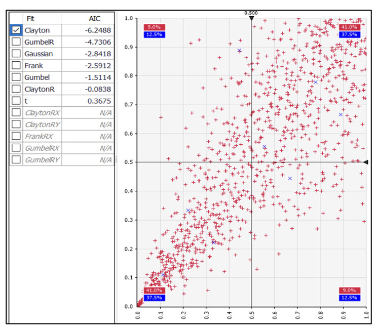
Plotting combinations of c and B values for each cedent generates the graph in Figure 5. It appears that the c and B values are not independent but have positive correlation. To keep this relationship in our frequency model, we introduced a copula dependence between each company’s c and B values.

Different subsets of data may be modelled with different copula functions. A bivariate Clayton copula is the best fit to our data as determined by the Akaike information criterion (AIC). Figure 6 shows resulting AIC rankings and data points from the fitted joint distribution.

We use the following notation for the cumulative density of a Clayton copula:

$$C(u,v) = \left( u^{- \theta} + v^{- \theta} - 1 \right)^{- \frac{1}{\theta}}$$

Modeling shape and scale dependence assuming a fixed value of θ results in posterior parameter estimates that fit the original data rather well. When plotted on a unit scale in Figure 7, one can clearly see the greater (left) negative tail dependence exhibited by both the observed data points and the Bayesian posteriors.

2.6. Implied Credibility and the Value of a Triangle

An implied credibility factor, $Z_{i}$, can be calculated for each cedent by specifying:

$$\lambda_{posterior}\lbrack i\rbrack = \left( 1 - Z_{i} \right)*\lambda_{prior}\lbrack i\rbrack + Z_{i}*\lambda_{empirical}\lbrack i\rbrack$$

where $\lambda_{empirical}\lbrack i\rbrack$ is the maximum likelihood estimate of the Poisson rate parameter based only on the i^th cedent’s data. In practice we found these values by running the frequency model with uninformative priors.

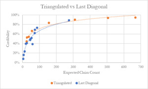
In Figure 8 we plot the implied credibility factor for each cedent against the expected number of claims based on the prior. Using the actual number of claims as a basis for credibility has a problem in that observing zero claims may actually contain significant information, for example if one hundred claims were expected to be observed. The chart also identifies cedents where a full claim count triangle was available as opposed to only the latest diagonal.

We can see that the majority of cedents had frequency credibility above 40%. A desirable and intuitive feature of the model is that it assigns higher credibility to cedents with triangulated data than those only providing losses from the last diagonal. No cedents with losses in triangulated form had frequency credibility falling below 40%. Cedents assigned the lowest credibility were all companies without triangles. This result is difficult to capture with traditional actuarial methods and is a distinct advantage of our Bayesian model.

Figure 9 plots the Weibull parameter joint probability densities for a certain company in our study. The graph plots a heatmap of the prior distribution in yellow and two posterior distributions in green and red. The range of parameters for the prior distribution is much wider and follows the gamma marginal distributions and Clayton copula described in Section 2.5. Both posterior distributions are concentrated within the company’s prior distribution.

The area in green represents the posterior distribution when only the last diagonal of excess claim count data is entered into the frequency model. What’s happening is that this company has, to the extent we can know, lower ultimate frequency than the mean of the prior distribution. When we observe the latest diagonal of observed claims, it is lower than expected. However, that could also be due to slow development. Without a triangle, the model must consider that possibility according to the prior distributions and Bayes’ Theorem. The result is the posterior distribution in green, which is very wide but populates mostly the “slow” region of the development parameter space (recall that higher values of c and B imply a slower development pattern).

Compare this to the area in red which is the frequency model’s posterior distribution using a full triangle of excess claim counts. Triangulated data produces more concentrated c and B values because of the increased certainty in the development pattern compared to only having the latest diagonal. What’s happening is that the model has much more information with which to reject the slow development hypothesis indicated by the low observed claim counts. Increasing the certainty of the development pattern while holding observed claim counts constant means that the model can be more certain that the ultimate frequency actually is lower than the prior mean, which is what occurred in this case.

Interestingly, the full triangle posterior is concentrated around the center of the prior but looks like an extreme outlier relative to the green distribution. The full triangle posterior can also be viewed as a Bayesian posterior with the green distribution as prior, with the marginal additional information being the claim counts in the interior of the triangle. This is what we mean by the “value of a triangle.” The triangle’s interior claim count data contains significant information about the pattern and ultimate frequency of a company’s large losses, a fact that is often overlooked or only accounted for subjectively in a reinsurance pricing analysis.

2.7. Case Study

A frequency data input file with two mock companies is provided in Appendix B. Only last diagonal data is given for Company 1 which has three excess claims over an 11-year period. Company 2 has 149 excess claims over the same period and data is available in triangulated form. A $500,000 threshold is used in this example. Parameters for the prior distributions are illustrative and programmed into the R/Stan codes in Appendix B.

Posterior means,^[2] standard deviations, distribution percentiles and MCMC convergence plots from the Bayesian model are presented in Figure 10. Company 2 has a smaller standard deviation around the posterior mean ultimate frequency due to a larger volume of claim count data and the availability of an excess claim count triangle. Using the formula in section 2.6, the implied credibility for Company 2 is 90% compared to 8% for Company 1. Note that implied credibilities are commensurate with the claim count versus credibility plot in Figure 8. However, they do not perfectly line up because prior distribution parameters for this case study are not the same.

Company 2 also has tighter ranges in the Weibull parameter posterior distributions. This is clearly seen in the MCMC convergence plots and evidenced by the relatively smaller standard deviation around posterior c and B means. There is increased certainty in the development pattern for Company 2 when compared to Company 1. A full triangle of excess claim counts provides the model with more confidence that the ultimate frequency for Company 2 is actually lower than the prior mean. The model can reject the hypothesis that lower-than-average observed claim counts are due to slow development.

On the other hand, Company 1 has low observed claim counts and only last diagonal data. The model does not have enough information to reject the slow development hypothesis. Therefore, a wider range of c and B values is contained in the posterior distributions.

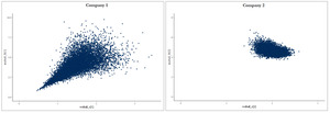
A visual comparison of joint probabilities densities is presented in Figure 11. The graph for Company 1 resembles the yellow prior distribution heatmap from Figure 9. With an implied credibility of only 8%, a wider range of distribution parameters makes sense. Low credibility assignments by the frequency model will yield posterior distributions that are closer to the prior distribution.

In contrast, the graph for Company 2 looks similar to the red area in Figure 9. A full triangle of excess claim counts produces more concentrated posterior joint probability densities. The model has more information with which to reject a larger number of parameter values.

This case study included two sample companies. However, the input files and code are set up to receive a more extensive number of cedents for simultaneous modeling. We encourage users to experiment with their own excess reinsurance portfolios.

3. SEVERITY MODEL

We also develop a Bayesian model for claim severity as depicted in Figure 12. We assume claims are Pareto distributed above the threshold. The shape parameter of the Pareto is allowed to differ by company. The Bayesian model weighs observed individual claim amounts against the prior distribution of each company’s shape parameter, and we use Stan/R/MCMC to calculate the posterior distribution, in particular the posterior mean, of each company’s pareto shape parameter.

One additional consideration is made to account for severity development, which is non-trivial in many long-tailed lines of business. We treat this in a simplified way by applying an age factor to the “ultimate” company Pareto $\alpha$. We stop short of the more complicated model in (McNulty 2017).

We assume there is no trend in the excess severity, as would be consistent with a Pareto distribution. Note that ground up severity trend is accounted for in the trend factors for excess frequency at the chosen threshold.

3.1. Gamma-Pareto Ultimate Severity

We use the following parameterization of the Pareto and gamma distributions with excess threshold T:

$${f(x;\alpha,\ T) = \left( \frac{\alpha T^{\alpha}}{x^{\alpha + 1}} \right);x > T }$$

$${f(x;\varepsilon,\ \beta)\ \sim\ \frac{\beta^{\epsilon}}{\Gamma(\epsilon)}x^{\varepsilon - 1}e^{- \beta x}}$$

Instead of using $\alpha,\beta$ as parameters of the gamma distribution we are utilizing $\varepsilon,\beta$ to avoid confusion with the Pareto $\alpha$.

3.2. Parameterizing the $\mathbf{\alpha}$ Prior

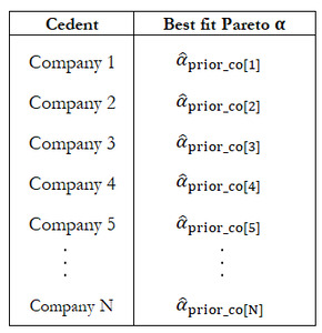
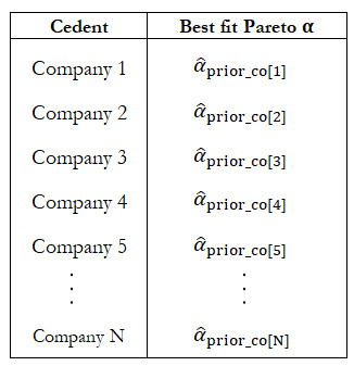
A prior mean for each company’s uncertain $\alpha$ Pareto shape parameter, denoted by $\widehat{\alpha}$, is established for each company in the portfolio. See Table 2. As with the ultimate frequency prior it is derived using an exposure rating method for this paper, but other methods of determining an a priori are also acceptable. The Pareto fitting exercise to determine each cedent’s $\widehat{\alpha}$ prior mean is only performed on the portion of the curve between T and $1M. Cedent data is right censored at policy limits. The most common commercial general liability limit in our data was $1M.

Similar to what we saw in the previous section on ultimate frequency, the array of best fit $\widehat{\alpha}$ prior means was well fit by a gamma distribution. The variance parameter from that fit, β, we then use as a universal value for β in the gamma prior distribution of each company’s uncertain Pareto $\alpha$ severity shape parameter. The mean of a gamma distribution is $\varepsilon/\beta$. Therefore, we have for each company:

$$\alpha_{prior\_ co\lbrack i\rbrack}\ \sim\ Г(\beta*{\widehat{\alpha}}_{prior\_ co\lbrack i\rbrack},\ \beta)$$

3.3. Pareto $\mathbf{\alpha}$ Development

If we observe a certain Pareto $\alpha$ in early ages, the ultimate $\alpha$ might not be the same because excess claim severity, for example in the $500K excess $500K layer, develops just as excess claim counts develop. A development pattern needs to be determined for the $\alpha$ parameter. A factor from this pattern is applied to $\alpha_{prior\_ co\lbrack i\rbrack}$ values, which are at ultimate, to bring the severity expectation to a level corresponding to the age of each observed claim.

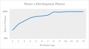
We assume a fixed $\alpha$ development pattern in the severity model. The pattern is obtained by creating an aggregated triangle of claim count data, excess of threshold T. Data is compiled from cedent loss listings that provide individual loss development. A development triangle of Pareto $\alpha$’s by year and age can be constructed from the excess claim count triangle. This can be done because given the distribution of individual claims in each cell of the triangle, a fitted Pareto shape parameter can be determined by maximum likelihood, moment matching, or fitting to percentiles such as the survival at $1M.

A cumulative α development pattern is then determined, similar to a selected development pattern from a triangle of link ratios. Unlike for frequency, we allow for no uncertainty in this pattern, or variation between cedents. In reality, there is uncertainty in this pattern. There is likely variation between cedents and there may even be correlation between a cedent’s frequency development and their severity development. These considerations would be good additions to a more complex model which we stopped short of in this paper.

A graph of the selected pattern used for our application of the severity model is shown in Figure 13.

3.4. Accounting for Policy Limit Capping

One complication that arises in some liability coverages in the US market is the presence of policy limits. Especially in a reinsurance application to large losses as in this paper, a significant portion of individual loss indemnity amounts excess of $500,000 will be exactly equal to the policy limit of $1 million.

This is censoring of the data and fitting distributions when presented with censored data is treated in Loss Models (Klugman, Panjer, and Willmot 2008). In a traditional maximum likelihood fitting exercise, to incorporate data censored above at T, instead of using the pdf value at T for those points the survival function is used which is the cumulative probability of the observation being greater than or equal to the censored value.

Our model uses Bayesian MCMC instead of maximum likelihood, but the principle is the same and the severity model code (see Appendix B) uses the complementary cumulative distribution function for the marginal probability associated with censored data points. The complementary cumulative distribution function is also known as the survival function and is one minus the CDF.

3.5. Estimating Posterior Distributions

The Bayesian model to estimate posterior distributions using the data is more straightforward for severity. Pseudo-code for the severity model would read as follows:

$$\text{Claims size} \sim \text{Pareto} (\text{T}, \alpha_{company\ i}\ * \text{age adjustment})$$

Only the company $\alpha$ is uncertain with its own distribution since the age adjustments are fixed values by age. In the actual model, extra steps are made to implement the policy limit censorship adjustment where the cumulative distribution function (CDF) is used for the marginal probability of censored values versus the probability distribution function (PDF) for uncensored values. See (Klugman, Panjer, and Willmot 2008) for more detail on fitting distributions to truncated and censored data.

3.6. Results

The Stan program simulates the posterior distribution of each company’s Pareto shape parameter. Although technically the compound Pareto mixture with variable $\alpha$ may be a more complex distribution (McNulty 2021), we simply took the mean of the posterior distribution of the $\alpha$ as a fixed value. This gave us a Pareto distribution for each company’s claims excess of T, which is a Bayesian blending of the prior distribution and the data, although not technically the full posterior distribution.

Interestingly we found that there was less “credibility” in the severity data than for frequency. The chart below shows the implied credibility factors, $Z_{i}$, such that:

$$\alpha_{posterior}\lbrack i\rbrack = \left( 1 - Z_{i} \right)*\alpha_{prior}\lbrack i\rbrack + Z_{i}*\alpha_{empirical}\lbrack i\rbrack$$

where $\alpha_{empirical}\lbrack i\rbrack$ is the maximum likelihood estimate of the Pareto shape parameter based only on the i^th cedent’s data. In practice we found these values by running the severity model with uninformative priors.

We can see in Figure 14 that the majority of cedents had severity credibility below 30%, and even in the case of the cedents with the most claims the credibility was at most 80%.

3.7. Case Study

A severity data input file with two mock companies is provided in Appendix B. The sample dataset was created and perturbed independently from the frequency dataset. Thus, the total number of claims and number of claims per year might not match the frequency input file. However, the information is more than sufficient to serve as a concrete example for the severity model.

Company 1 has five excess claims over a 10-year period. Company 2 has 64 claims over a 14-year period. As with the frequency model case study, a $500,000 threshold is used in this example. Parameters for the prior distributions are illustrative and programmed into the R/Stan codes in Appendix B.

Posterior means, standard deviations, distribution percentiles and MCMC convergence plots from the Bayesian model are in Figure 15. In the severity model R code shown in Appendix B, the company prior $\alpha$ values are shown as (0.95, 1.05). Company 1, which has barely any data, results in a posterior mean of 0.95 after running the model, i.e., exactly the same as the prior. This is consistent with the expected implied credibility based on Figure 14 of 0% for such a low claim count.

Company 2, on the other hand, has a significant amount of data that would result in an implied credibility of perhaps 30% to 40% weight towards the empirical Pareto $\alpha$ (assuming a similar credibility profile as Figure 14 and a claim count of 64), and away from the prior $\alpha$ of 1.05 as specified in the code. The posterior mean $\alpha$ as shown in Figure 15 is 1.21, meaning that Company 2 displays lower than average severity in the excess layer, after adjusting for policy limits and severity development.

As with the frequency model case study, input files and R/Stan codes are set up to receive a more extensive number of cedents for simultaneous modeling. The model is set up to handle entire portfolios or large subsets of reinsurance portfolios.

3.8. Treatment of ALAE

The model developed to this point in Section 3 has concerned indemnity only. In the US market, claims in long tailed lines of business often incur significant loss adjustment expense, or ALAE, in addition to indemnity. A full model of large casualty losses for reinsurance in the US needs to have a provision for ALAE, which can be treated as included in-addition or pro-rata with loss for determining the reinsured portion of ALAE.

The standard way of modeling ALAE would be to multiply every indemnity loss by a factor, for example 1.2, to gross up to a loss amount with ALAE. This is what the authors did in implementing the method in this paper for use in reinsurance pricing. There is a more realistic, although also more complicated, model for ALAE which fits a separate distribution for ALAE amounts, and then models the bivariate distribution of ALAE and indemnity with a copula. That model would be beyond the scope of this paper but see, e.g., (Micocci and Masala 2009) for more information.

4. COMPARISON TO EXISTING METHODS

The defining features of the model developed in this paper, and the reason why we believe it is novel research, is that we address both problems of severity development and uncertainty in the claim count development in a Bayesian large loss model. We wanted to highlight some other papers that come the closest and compare the differences and similarities between the methods.

4.1. Cockroft/Buhlmann

Cockroft, in his 2004 paper (Cockroft 2004), develops what we would call a classical credibility treatment for excess of loss claims. He derives the formulas for applying Buhlmann best linear approximation to the Bayesian posterior mean in the case of a compound Gamma-Poisson, Gamma-Pareto model.

There are a few elements developed in our paper which we believe are advantages. First, the Cockroft treatment does not allow for claim development, so it is more suitable for short-tailed lines of business. For long-tailed lines, where claim development and uncertainty in the development pattern are keys to estimating the mean, we suggest incorporating the methods from this paper.

Trend is another very important parameter in any reinsurance pricing. Cockroft’s paper assumes all data is trended before fitting the model. In practice this would make it difficult to include trend as an uncertain parameter in a Bayesian analysis. We also chose to use fixed trend factors, but since the trend factor is explicitly used in our frequency model with untrended data, we could easily give the trend a prior distribution. This would allow for uncertainty in the posterior and cedent specific differentiation.

On the severity side, Cockroft does not address policy limit capping, whereas we have explicitly incorporated it into our severity model and provided code for practitioners who may have policy limit censored data.

Finally, the Buhlmann method is fundamentally concerned with a best estimate of the mean and develops a best linear approximation. Cockroft goes further by deriving full posterior distributions for some quantities of interest but not all. Since R and Stan are simulation based, it would be easy to define the mean layer loss as a variable and observe the MCMC samples of the full distribution of the posterior. It’s also not clear that in the case of reinsurance, with heavily right-skewed distributions, that the best linear approximation to the posterior mean is a good approximation.

4.2. Barnett

The authors wanted to highlight (Barnett 2020) as it is one of the only papers we found that addressed the issue of development in a Bayesian large loss or reinsurance excess of loss model. In order to stay practical, the author develops the model in tables and spreadsheets which makes it more usable but probably limits the complexity of the model. For example, the model does not consider uncertainty in the development pattern, which we believe to be a key factor in reinsurance excess of loss estimation.

Note that Bayesian reserving models or models for estimating ground up loss ratios which do incorporate uncertainty in the development pattern have been well developed by, e.g., (Zhang, Dukic, and Guszcza 2012) and (Clark 2003).

4.3. Mildenhall

Mildenhall’s 2006 paper, “A Multivariate Bayesian Claim Count Development Model With Closed Form Posterior and Predictive Distributions” (Mildenhall 2006) introduced a completely new model, breaking the Buhlmann mold. The model uses Gamma-Poisson ultimate claim counts and a multinomial Dirichlet claim count development distribution.

The greatest achievement of this paper is that it addresses the fundamental question of weighing uncertainty in the ultimate frequency against uncertainty in the development pattern. The author includes a very enlightening chart on page 472 that shows where established reserving methods lie on the spectrum of the relative size of the uncertainty in those two parameters.

In contrast to Mildenhall, we prefer the simpler Weibull development pattern distribution to the multinomial Dirichlet for several reasons. The Weibull is a 2-parameter distribution, and as discussed above there are intuitive visual interpretations of the parameters. This can be beneficial when priors are specified using judgment. In contrast, the Dirchlet has as many parameters as there are development ages (minus one) and so it would be difficult to intuitively judge or visualize the prior. This also leads the total model to have n + 2 parameters when there are n time periods as stated in Section 7 of the paper, whereas the model presented in this paper has a total of seven^[3] parameters independent of how many time periods there are.

Another advantage of the Weibull is that it is continuous which means that we are easily able to incorporate information from a partial diagonal of a triangle or data at different ages, such as a 12-month triangle with a six-month latest diagonal which is quite common in reinsurance practice. The multinomial Dirichlet is discrete with each point representing one time period which would typically be a year. It’s not clear how a practitioner would deal with data that is at different ages.

Lastly, consider the following statement from the Mildenhall paper on page 468:

“Proposition 4 shows the predictive distribution does not depend on the individual observed values b1, •.. , bt but only on their sum b(t) = b1 +·· ·bi. Thus, the GPDM model has a kind of Markov property that the future development depends only on the total number of claims observed to date, and not on how those claims were reported over time.”

The authors of this paper would argue that the Markov property is unintuitive for insurance losses. The times at which various claims have been reported in the past contains valuable information about future development. This was demonstrated in Section 2 which showed that the frequency model can provide a much more concentrated posterior for the development pattern in the case of a cedent who provides a full triangle. If only the latest diagonal or total number of claims reported to date mattered in the model, i.e., the model demonstrated the Markov property, then we would get the same results when giving the full triangle or simply the latest diagonal. We view the absence of the Markov property to be a fundamental advantage of our model.

functions {
  real clayton_log_pdf(real u, real v, real theta) {
    return log((1+theta)*pow(u*v,-1-theta)*pow(pow(u,-theta)+pow(v,
    -theta)-1,-((2*theta+1)/theta)));
  }
}
data {
  int<lower=0> N_obs;
  int<lower=0> N_obs_start;
  int<lower=0> N_obs_end;
  int<lower=0> N_companies;
  real beta;
  real premium[N_obs];
  real co_lambda_prior[N_companies];
  int<lower=0> year[N_obs];
  real<lower=0> obs_start[N_obs];
  real<lower=0> obs_end[N_obs];
  int<lower=0> company[N_obs];
  int<lower=0> incr_claims[N_obs];
}
parameters {
real<lower=0> company_freq[N_companies];
real<lower=0> weibull_c[N_companies];
real<lower=0> weibull_B[N_companies];
}
transformed parameters {
real pois_lambda[N_obs];
real normalized_weibull_c[N_companies];
real normalized_weibull_B[N_companies];
	for( i in 1 : N_obs ) {
		pois_lambda[i] = company_freq[company[i]] * premium[i]
        * (exp(-pow((obs_start[i]/weibull_B[company[i]]),
        weibull_c[company[i]])) - exp(-pow((obs_end[i]/
        weibull_B[company[i]]),weibull_c[company[i]])))
        *pow(1/1.1,2022-year[i]);	
	}
  for ( i in 1 : N_companies) {
    normalized_weibull_c[i] = gamma_cdf(weibull_c[i], 13,9);
  }
    for ( i in 1: N_companies) {
    normalized_weibull_B[i] = gamma_cdf(weibull_B[i], 8,2);
  }
}
model {
for (i in 1:N_companies){
	weibull_c[i] ~ gamma(13,9);
}
for (i in 1:N_companies){
	weibull_B[i] ~ gamma(8,2);
}
for (i in 1:N_companies){
  target += clayton_log_pdf( normalized_weibull_c[i],
  normalized_weibull_B[i], 2.75 );
}
for (i in 1:N_companies){
	company_freq[i] ~ gamma(beta*co_lambda_prior[i],beta);
}
for (i in 1:N_obs){
	incr_claims[i] ~ poisson(pois_lambda[i]);
  }
}
generated quantities {
}

data {
  int<lower=0> N_claims;
  int<lower=0> N_years;
  int<lower=0> N_ages;
  int<lower=0> N_companies;
  real threshold;
  real beta;
  real <upper = 1000000> incurred[N_claims];
  real age_factor[N_ages];
  real co_alpha_prior[N_companies];
  int<lower=0> year[N_claims];
  int<lower=0> age[N_claims];
  int<lower=0> co[N_claims];
  int<lower = 0, upper = 1> censored[N_claims];
}
parameters {
real<lower=0> co_alpha[N_companies];
}
transformed parameters {
real claim_alpha[N_claims];
	for( i in 1 : N_claims ) {
		claim_alpha[i] = co_alpha[co[i]] * age_factor[age[i]];		
	}
}
model {
for (i in 1:N_companies){
	co_alpha[i] ~ gamma(beta * co_alpha_prior[i], beta);
}
for (i in 1:N_claims){
	if (censored[i]) {
      			target += pareto_lccdf( incurred[i] | threshold,
                claim_alpha[i]);  
    		} else {
      			target += pareto_lpdf( incurred[i] | threshold,
                claim_alpha[i]);
  		}
}
}
generated quantities {
}

library(dplyr)
library(distr)
library(fitdistrplus)
library(actuar)
library(rstan)
library(readr)
library(rstudioapi)
library(bayesplot)
library(ggplot2)
#setwd
setwd("C:/folder")
##import data
data <- read_csv("freq data.csv", 
                            col_types = cols(company = col_integer(),
                                             year = col_integer(),  
                                             premium = col_double(),
                                             obs_start = col_double(),
                                             obs_end = col_double(),
                                             incr_claims = col_integer()))
##make the data list
attach(data)
##co priors are for the prior ultimate freq per 10M premium for each company
co_lambda_prior <- c(1.5,2.5)
##universal beta param for ultimate claim count gamma distributions
beta<- 9
##transform data
##our frequencies are stated per $10M of premium so rescale the premium
data to match
premium<-premium/10000000
data_list <- list(  
  year = year,
  obs_start = obs_start,
  obs_end = obs_end,
  incr_claims = incr_claims,
  company = company,
  premium = premium,
  co_lambda_prior = co_lambda_prior,
  beta = beta,
  N_obs = length(incr_claims),
  N_obs_start = max(obs_start),
  N_obs_end = max(obs_end),
  N_companies = max(company))
##run stan
fit<- stan(file = 'stan code freq model.stan', data=data_list, iter=10000,
chains = 4, cores = 4, seed =123)
## plot output
print(fit, pars=c("company_freq", "weibull_c", "weibull_B"))
traceplot(fit, pars=c("company_freq", "weibull_c","weibull_B"),
inc_warmup = TRUE)

library(dplyr)
library(distr)
library(fitdistrplus)
library(actuar)
library(rstan)
library(readr)
#setwd
setwd("C:/folder/")
##import data
data <- read_csv("sev data.csv", 
            col_types = cols(age = col_integer(), 
            incurred = col_double(), co = col_integer(), year = col_integer()))
##make the data list
attach(data)
##age factor is for relativity of early alphas to ultimate (multiplicative)
## must satisfy len(age_factor) = N_ages
age_factor <- c(.5, .75, .9, .95,1,1,1,1,1,1, 1, 1, 1,1, 1, 1)
##co priors are for the prior ultimate alpha for each company
co_alpha_prior <- c(0.95,1.05)
##universal beta param for all gamma distributions
beta<- 40
##implement 1M upper censoring on incurred
incurred[incurred>1000000]<-1000000
censored <- incurred==1000000
data_list <- list(  
  incurred = incurred,
  year = year,
  age = age,
  co = co,
  N_claims = length(incurred),
  N_years = 16,
  N_ages = 16,
  N_companies = 2,
  threshold = 500000,
  age_factor = age_factor,
  co_alpha_prior = co_alpha_prior,
  beta = beta,
  censored = censored
)
##run stan
fit<- stan(file = 'stan code sev model.stan', data=data_list, iter=2000,
chains = 1, cores = 4)
## plot output
print(fit, pars=c("co_alpha"))
traceplot(fit, pars=c("co_alpha"), inc_warmup = FALSE)