Ultimate Loss Reserve Forecasting Using Bidirectional LSTMs

1. Introduction

1.1. The life of a claim

A claim is a policyholder’s request for financial indemnification from an insurance company after a loss causing event. When a claim is brought to the knowledge of the insurance company with whom the claimant has an insurance policy, the claim is said to have been reported. The time elapsed between the occurrence date of the event producing the claim and the date which the claim is reported is called the reporting delay (Amin et al. 2020). Once the claim has been reported to the insurer, a claim file is opened, and the claim development process begins where the insurer takes the necessary steps to process and settle the claim. Once the claim is settled, i.e. the claim is not expected to develop any further, the claim is then closed (Closed claims can be reopened if necessary). The time between the date the claim is reported and the date when the claim is closed is called the settlement delay (Amin et al. 2020). The settlement delay can be separated into time periods, called lag periods. At the end of each lag period, we can observe the state of the claim in terms of how much it has developed or changed over the previous lag periods. Due to the settlement delay that is inherent in any claim development process, the insurer at any time can have claims that are open and not fully developed. The state of development correlates with how far back in time the relevant claim was reported. The further back in time a claim was reported, the longer time it has had to develop, which can cause the oldest claims to be fully developed and closed.

To better manage its open claims, insurers often aggregate claims by the accident year (or the underwriting year), the development year, or the calendar year (or the accounting year) (Radtke 2016, 242). The variables used to measure aggregate claims are cumulative paid losses, loss reserves, or incurred losses (Radtke 2016, 243). The cumulative paid losses for a particular claim at some time $k$ represents the total dollar amounts the insurer paid with regards to the claim up until time $k.$ The loss reserves for a particular claim at some time $k$ represents the insurer’s estimate of the size of the unpaid claim remaining at time $k.$ The incurred losses for a particular claim at some time $k$ represents the insurer’s estimate of the size of the claim increment from time $k-1$ to time $k.$ This paper focuses on loss development of cumulative paid losses because cumulative paid losses tend to be more stable in the loss development pattern. Specifically, cumulative losses almost always follow a monotonically increasing function over time, which makes predicting cumulative losses an easier task.

1.2. Data Representation for Loss Reserving

Data representation is an important aspect of loss reserving. Not only does it impact how the reader perceives data, the choice of how data is represented also impacts the choice of methods that can be used to develop loss data. The traditional approach to representing loss reserving data is a loss development triangle where loss development data are grouped according to Accident Year (AY) and Development Year (DY). For example, suppose that we are looking at some hypothetical loss data across 6 accident years (2000-2005), over 6 development years. If we regard the x-axis as development years and y-axis as accident years, we arrive at this tabular format shown in Table 1.

For AY 2004, the only observed losses are from development years 2004 and 2005, because no data for AY 2004 exists for any time before 2004. Thus, the earliest theoretical observation for any accident year exists on the leading diagonal, rendering any cells below this diagonal to be empty. A more efficient method of representing loss development data would be to change the development years from absolute to relative years. Development years defined in this manner refer to the $n^{\text{th}}$ year period after year of the accident. For example, DY 1 refers to the time period between 1 and 2 years after the accident took place. Rearranging Table 1 in this fashion would yield Table 2. This is an example of a run-off table (Schmidt 2016, 248).

The counter diagonal gives the latest observable data (cumulative paid loss), for each accident year. The unobserved cumulative paid losses can be found below the counter diagonal (this data is currently empty). The final relative development period for each accident year gives the ultimate losses. These losses are matured losses which can be regarded as having reached full development. The objective of this paper is to predict these ultimate paid cumulative losses.

1.3. Loss Reserving Methods

Although there are many methods for estimating property/casualty loss reserves, there are a few methods that are most commonly used. The most well-known method is the chain ladder method and there are many variations of the chain ladder method. Briefly, under the chain ladder method, the ratio of cumulative incurred losses (called the loss development factor) is calculated for successive loss development years. Assuming we have a loss development triangle with at least some fully developed loss data, the average loss development factors across the accident years are used to calculate cumulative claim development factors, which are then used to project ultimate loss. The loss reserve is the difference between the projected ultimate loss and the paid incurred loss. In general, loss reserving methods can broadly be classified as being based on a parametric model or a non-parametric model. Traditionally, parametric models have been used due to ease of interpretation and calculation. Models such as the over-dispersed Poisson, negative binomial, lognormal, and gamma models have been shown to be capable of replicating the chain ladder based reserving methods (England and Verrall 2002, 11). These models are centered around estimating some parameters such as the means and the variances, either by accident year or loss development period, or both. Doing so condenses the number of parameters used by the model and helps in identifying the “ingredients” that went towards estimating the losses. However, the assumptions needed in the process of constructing parametric models can limit the predictive power of the model. Particularly in the case where the underlying factors which drive the dynamic relationships between data is not well understood, non-parametric models can outperform parametric models (Mills and Markellos 2008, 224).

A common feature of established loss reserving methods is their reliance on the existence of a sufficiently long loss run-off triangle. Ramsay (2007, 462) developed a non-parametric loss reserving method/process to assist them with their “best guess” in the early years of development and with loss reserving in general. Ramsay’s method is fundamentally different from previous loss reserving methods. Given that losses are settled in $n$ years, Ramsay’s method assumes the evolution of the incremental incurred loss over development years is the result of a random split of the ultimate loss for that accident year into $n$ separate pieces of losses, which are then ordered from largest to smallest. The largest incremental loss is observed in the first development year, the second largest incremental loss is observed in the second development year, etc., so that the smallest incremental loss is observed in the last development year. Ramsay’s approach requires no prior knowledge of the distribution of the ultimate loss or of the actual cumulative incurred loss. In addition, it uses little or no loss development data.

Our Objective: To use deep learning to provide a loss reserving tool for actuaries to use loss development data to produce more efficient and accurate estimates of property and casualty loss reserves. Although we will use order statistics, our approach is different from Ramsay (2007).

2. Machine Learning and Deep Learning

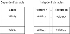
In order to properly understand what deep learning is, we must briefly visit what machine learning is, since the former is a subset of the later. Central to the debate of what machine learning is, is the question, “Rather than programmers crafting data-processing rules by hand, could a computer automatically learn these rules by looking at data?” A distinct advantage that machine learning has over classical statistics is the ability of machine learning models to handle data of a large volume, which can sometimes be a challenge to classical statistical methods (Chollet 2018). Machine Learning can be broadly divided into three areas: supervised learning, unsupervised learning, and reinforcement learning. In supervised learning, data fed into a machine learning algorithm are divided into dependent and independent variables. It is called supervised learning because the dependent variables act as a guide, in helping identify the patterns that exist in the data. The unsupervised learning process has no dependent variable to measure the learning process against. Instead, the features of data are observed and similarities between data points are determined (Hastie, Tibshirani, and Friedman 2017). The last type of learning is reinforcement learning; the process of using a reward structure to make the algorithm learn the best course of action under a given set of circumstances (Sutton and Barto 2018). Supervised learning can be further broken down into problems that involve regression or problems that involve classification, where the objective of regression problems is to predict some value such as a reserve forecast and the objective of classification problems is to identify if an outcome belongs to certain class, such as if a loss ratio will exceed a certain threshold. Since many problems that actuaries deal with involve some level of financial prediction, most actuarial problems can be viewed as regression problems. Expressing actuarial problems as regression problems makes them suitable to be solved using machine learning (Richman 2020, 230–58).

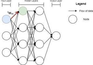
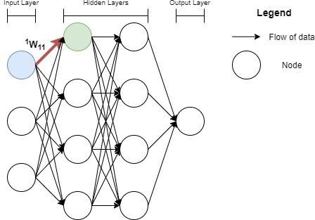
Deep learning is a subset of machine learning which learns increasingly more meaningful representations of data in a more hierarchical fashion. You could look at other forms of machine learning as “shallow learning,” since they do not use as many hierarchical layers to learn about meaningful patterns in the data that they receive (Chollet 2018). The key advantage of learning patterns in a hierarchical fashion is that at various levels of abstraction, various patterns can be discovered. It is easier to discover more granular patterns present in data this way. A typical implementation of a deep learning model is via a neural network, as shown in Figure 1. There are many different flavors of neural networks, each being unique in its own way. For the purpose of simple illustration of the concept, we will present a figure of a neural network, which utilizes a fully connected feed-forward neural network structure.

Figure 1.Fully Connected Feedforward Neural Network

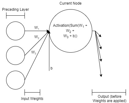
In the example of a neural network given in Figure 1, each node receives input from all nodes of the previous layer. This network has an input layer $I,$ that takes in 3 inputs, $I \in \mathbb{R}^{3}.$ Similarly, the output layer $O,$ utilizes 1 node to output 1 value, $O \in \mathbb{R}^{1}.$ Barring the input layer, each node of each layer implements a linear regression function. Figure 2 shows the workings of a node up close.

Figure 2.Functioning of a node

As mentioned before, each node (other than the input nodes) receives output from the preceding layer of nodes, as an input into it (Zhang, Lipton, Li, and Smola 2021). The inputs are each weighted differently. Therefore, we can represent the weighted inputs into the node as $w_i \beta_i,$ where $w_i$ represents the $i^{\text{th}}$ weight, $\beta_i$ represents the $i^{\text{th}}$ input into the node, for $i = 1,2,\cdots,n$ and $n$ represents the $i^{\text{th}}$ input. These inputs also contain a bias term $b.$ The data that is aggregated inside the node this way, is finally fed through an activation function to get the final output:

$$\text { node output }=f\left(b+\sum_{i=1}^{n} w_{i} \beta_{i}\right) \tag{1}$$

where f (x) is an activation function for x ∈ R. A typical activation function used would be the “sigmoid” activation function^[1]:

$$f(x)=\frac{1}{1+\mathrm{e}^{-x}}\tag{2}$$

where $x \in \mathbb{R}.$ As mentioned before, there are many flavors of neural networks and the type of network that will be the focus of this paper is a supervised neural network, where data is fed in the form of dependent variables (features) and independent variables (labels).

Figure 3.The general structure of a dataset of with n features and m rows

Features are fed into the input layer and passed forward through the network, where at the end of the network (the output layer), predictions are made. These predictions are then evaluated by a loss function, which aims to calculate the error of the predictions. Typically, the mean squared error function is used (Alzubaidi et al. 2021, 20):

$$L(\hat{y}, y)=\frac{1}{2 N} \sum_{i=0}^{N}(\hat{y}-y) \tag{3}$$

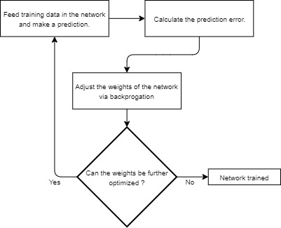
where $\hat{y}$ is the predicted output and $y$ is the actual output. Optimizing the loss function means that the predicted output of the neural network needs to be as close as possible to the actual output of the data set. This process of optimizing is called training the network. As mentioned earlier, each neuron of each layer of the neural network has its own respective weights that regulate the strength of incoming signals from the preceding layers and biases. Therefore, we need to change these weights and biases through a process known as backpropagation, where all of the network’s weights and biases are optimized, with respect to a given loss function (Zhang, Lipton, Li, and Smola 2021). The goal here is to minimize the given loss and in turn find the weight and bias settings that enable this said minimization:

$$w^{\prime}, \beta^{\prime}=\arg \min _{w, \beta} L(\hat{y}, y) \tag{4}$$

where $w^{\prime}$ and $\beta^{\prime}$ are network optimized weights and biases. Through backpropagation and using the multidimensional gradient descent method, we are able to iteratively adjust the weights and biases of the network, taking into consideration the sensitivity of each weight and bias, in relation to the loss function. The goal is to optimize weights in proportion to the impact that their change has on minimizing the loss. We can represent the optimization task on a given weight as the following partial derivative:

$$\Delta^{(k)} w_{i j}=-\eta \frac{\partial L}{\partial^{(k)} w_{i j}} \tag{5}$$

where $\Delta^{(k)} w_{i j}$ represents the change in given weight, $k$ represents the layer which the weight belongs to, $i$ is the destination node (the node which receives the weight), $j$ is the origin node (the node which outputs the weight), and $\eta$ is the learning rate (a tunable hyperparameter of the model). Thus the newly optimized weight can be represented as:

$${ }^{(k)} w_{i j}^{\prime}={ }^{(k)} w_{i j}+\Delta^{(k)} w_{i j} \tag{6}$$

Figure 4.A demonstration of a weight

We can represent the optimization process to include all weights and biases as:

$$\Delta \mathbf{W}=\left(\Delta^{(1)} \mathbf{W}, \Delta^{(2)} \mathbf{w}, \ldots, \Delta^{(p)} \mathbf{w}\right) \tag{7}$$

where $\Delta \mathbf{W}$ is a $(m \times n \times p)$ 3D matrix composed of individual matrices containing the changes in weights and biases, for each layer of the network, and, for $r = 1,2,\cdots,p,$

$$\Delta^{(r)} \mathbf{w}=\left[\begin{array}{cccc} \Delta^{(r)} w_{11} & \Delta^{(r)} w_{12} & \cdots & \Delta^{(r)} w_{1 n} \\ \Delta^{(r)} w_{21} & \Delta^{(r)} w_{22} & \cdots & \Delta^{(r)} w_{2 n} \\ \vdots & \vdots & \cdots & \vdots \\ \Delta^{(r)} w_{m 1} & \Delta^{(r)} w_{m 2} & \cdots & \Delta^{(r)} w_{m n} \end{array}\right] \tag{8}$$

and $p$ represents the maximum number of layers in the network. For simplicity, we assume that the number of nodes for each layer is fixed, and therefore the maximum number of origin nodes and maximum number of destination nodes are the same for any particular layer. Therefore, at each iteration, a new 3D matrix $\mathbf{W}^{\prime}$ is created:

$$\mathbf{W}^{\prime}=\mathbf{W}+\Delta \mathbf{W} \tag{9}$$

where

$$\mathbf{W}=\left({ }^{1} \mathbf{w},{ }^{2} \mathbf{w}, \ldots,{ }^{p} \mathbf{w}\right) \tag{10}$$

$$\mathbf{W}^{\prime}=\left({ }^{1} \mathbf{w}^{\prime},{ }^{2} \mathbf{w}^{\prime}, \ldots,{ }^{p} \mathbf{w}^{\prime}\right) \tag{11}$$

and, for $r = 1,2,\cdots,p,$

$$(r) \mathbf{w}=\left[\begin{array}{cccc} (r) w_{11} & (r) w_{12} & \cdots & (r)_{1 n} \\ (r) w_{21} & (r) w_{22} & \cdots & (r)_{2 n} \\ \vdots & \vdots & \cdots & \vdots \\ (r)_{21} & (r) w_{m 2} & \cdots & (r)_{m n} \end{array}\right] \tag{12}$$

$${ }^{(r)} \mathbf{w}^{\prime}=\left[\begin{array}{cccc} { }^{(r)} w_{11}^{\prime} & { }^{(r)} w_{12}^{\prime} & \cdots & { }^{(r)} w_{1 n}^{\prime} \\ { }^{(r)} w_{21}^{\prime} & { }^{(r)} w_{22}^{\prime} & \cdots & (r)^{\prime} w_{2 n}^{\prime} \\ \vdots & \vdots & \cdots & \vdots \\ (r) w_{m 1}^{\prime} & (r) w_{m 2}^{\prime} & \cdots & \left.{ }^{(r}\right)_{m n}^{\prime} \end{array}\right] \tag{13}$$

where $\mathbf{W}$ and $\mathbf{W}^{\prime}$ represent the 3D matrix of optimized weights and biases from the last iteration of the network optimization, and the 3D matrix of the newly optimized weights and biases, respectively. The weights and biases are adjusted, until the weights of the $\Delta\mathbf{W}$ matrix cause the training loss to begin increasing, instead of decreasing. This can be represented as shown in Figure 5.

Figure 5.Neural network training process

3. Recurrent Neural Networks (RNNs)

As is evident by the introduction, loss development has a strong temporal component. Therefore, any deep learning model that is used to make loss development predictions needs to take this aspect of the data into account. For this reason, recurrent neural networks are a worthy choice to consider. The basic premise of these types of networks is the reliance of a past sequence of data to make a prediction. This can be represented as follows (Zhang, Lipton, Li, Smola, et al. 2021): the conditional probability of observing $x$ at time $t$ (i.e., $x_t),$ given previous observations at times $1, 2, \cdots, t - 1$ can be written as $\operatorname{Pr}\left(x_{t} \mid x_{t-1}, x_{t-2}, \ldots, x_{1}\right).$ As it is generally prohibitively costly to store all information of a given sequence in memory, we therefore can retain the partial information given a certain subset of this sequence. This partial information subset can be identified as the hidden state, $h_{t-1}.$ This leads to the conditional probability given the partial information as $\operatorname{Pr}\left(x_{t} \mid h_{t-1}\right).$ The hidden state itself can be represented recursively as:

$$h_{t-1}=f\left(x_{t-1} \mid h_{t-2}\right) \tag{14}$$

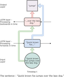
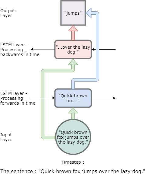
where $x_{t-1}$ is the observation at time $t - 1$ and $h_{t-2}$ is the hidden state at time $t-2.$ In comparison to the node described before, a node of a RNN can be “unrolled” in time due to it having this hidden state. An intuitive illustration of how an RNN processes sequential data by remembering input from previous timesteps is depicted in Figure 6.

Figure 6.How an RNN processes sequential data

As Figure 6 illustrates with the sentence “Quick brown fox jumps over the lazy dog,” at each time step, information from previous timesteps is used to predict the output at that time step. Note that the hidden state can only contain a finite amount of information and therefore tends to hold past information only within a certain time frame. Mathematically speaking, the introduction of hidden states now implies that there are more weights and biases to optimize. If we visualize the weights as matrices - for feedforward neural networks, we only have matrices with weights relating to the current time, $t.$ With a hidden state, each weight will now have a hidden state version of it.

We can represent the flow of data of RNN in matrix notation in the following manner:

$$\mathbf{H}_{t}=\alpha\left(\mathbf{X}_{t} \mathbf{W}+\mathbf{H}_{t-1} \mathbf{W}_{h}\right) \tag{15}$$

where $\mathbf{H}_{t}$ is the output vector of the hidden layer at time $t,$ $\mathbf{X}_{t}$ is the input vector at time $t,$ $\mathbf{H}_{t-1}$ is the output vector of the hidden layer from time step $t - 1$ (also the hidden state at time $t),$ $\mathbf{W}$ is the weight matrix, of which the first layer is multiplied by $\mathbf{X}_t.$ $\mathbf{W}_h$ is the weight matrix of the hidden layers, of which the first layer is multiplied by $\mathbf{H}_{t-1},$ which is the same matrix discussed in Section 5, and $\alpha$ is the symbol of the activation function used in the respective layer. As $\mathbf{W}$ and $\mathbf{W}_h$ are composed of matrices $\mathbf{W}^r$ and $\mathbf{W}^r_h,$ respectively, where $r$ refers to a layer of the neural network and $p$ is the maximum number of hidden layers in the network), equation 15 can also be written as:

$$\mathbf{H}_{t}=\alpha\left(\left(\left(\mathbf{X}_{t} \mathbf{W}^{0}\right) \cdots\right) \mathbf{W}^{p}+\left(\left(\mathbf{H}_{t-1} \mathbf{W}_{h}^{0}\right) \cdots\right) \mathbf{W}_{h}^{p}\right) \tag{16}$$

where $\mathbf{X}_{t} \in \mathbb{R}^{d},$ $\mathbf{H}_{t-1} \in \mathbb{R}^{d},$ and the following $d \times d$ matrices: $\mathbf{W}=\left\{W_{i j}\right\}$ and $\mathbf{W}_h =\left\{W_{h: i j}\right\}$ for $i, j \in\{1,2, \ldots, d\}.$

Figure 7.Weights of a feedforward network, without recurrent connections

Figure 8.Weights of a feedforward network, with recurrent connections

4. Long Short-Term Memory Cell (LSTM)

A recent innovation in RNN has been Long Short Term Memory (LSTM). The fundamental reason for LSTM preference in sequence prediction is the ability of LSTM cells to learn relevant information in long input sequences (Sherstinsky 2020, 1).

As a LSTM cell is fed with a sequence of data, it continuously changes its state and in doing so, it changes its long-term and short-term memory. Figure 9 shows more of the anatomy of a LSTM cell. The main idea behind an LSTM cell is its ability to overcome the “short-term” memory issues of the plain RNN architecture. How it accomplishes this is by having two dedicated parts in its memory, one for short and one long term pattern identification. “Cell state” refers to the long-term memory and the “Hidden state” refers to the short term memory. As seen in Figure 9, there is a sinusoidal wave, which has a sudden amplitude change at every 1000 time steps. With plain RNNs, the sine wave that repeats every time step will be learned well but the sudden change at the longer time interval will be missed. LSTMs however do not suffer from this fate.

Figure 9.How LSTM handles short and long term dependencies

As shown in Figure 10, bidirectional LSTMs consume data in both directions. This helps to establish context better because not only previous timestamps are used, but also data from future time stamps can also be used to predict outcomes. As shown with the dummy sentence, “Quick brown fox jumps over the lazy dog,” the prediction uses data fed in both directions: backwards and forwards (Basaldella et al. 2018, 182–83). It is important to note that bidirectional data feeding only happens during training. During inference, we do not know what the future sequences are for certain.

Figure 10.How bidirectional LSTMs get data

5. Main Research Idea

5.1. The Crux of the problem

Let us consider a set of independent companies labeled $\{0, 1, \cdots, b\}.$ Each company provides cumulative loss development (CLD) data, with consecutive accident years (AYs) labeled $\{0, 1, \cdots, m\}$ and development years (DYs) labeled $\{0, 1, \cdots, n\}$ and $m \geq n$ where $m$ is the current year. Let $C_{kij}$ denote the cumulative paid losses for k^th company, originating in the i^th accident year and at the j^th development year, where $i \in\{0,1, \ldots, m\},$ $j \in\{0,1, \ldots, n\},$ and $k \in\{0,1, \ldots, b\}.$

Consider Table 3 which shows the cumulative paid losses of a P&C company. For the purposes of generalizing this table over a number of the companies of the same line of business, let’s consider the $k^{\text{th}}$ company. Claims for each accident year develops over $n$ development years (also called lags). After the $n^{\text{th}}$ lag period from the accident year, we assume that claims from that respective accident year are considered closed, i.e.: the claims have matured and reached the ultimate losses so that no more claims can arise from accidents that took place in this specific accident year (Radtke, 2016). We consider the most recent accident year which we have data as the $m^{\text{th}}$ accident year. This implies that for the $m^{\text{th}}$ accident year, we only have claims information for a single lag period, i.e., losses have only had one time period to develop. Therefore, for any accident year, $h (h < m),$ it is easy to see that we have $n - h$ unobserved loss developments periods. This means that for the $h^{\text{th}}$ accident year, the last observable cumulative paid loss is $C_{k,h,n-h}$ (Schmidt 2016). If $m = n,$ this gives us a cumulative paid loss development run-off triangle, for the $k^{\text{th}}$ company, as shown in Table 4. Note that Table 4 shows a loss triangle that an insurance company typically faces. As can be seen, certain accident years have unobserved cumulative paid losses and the first unobserved cumulative paid loss occurs at $C_{k,h,n-h+1}.$

Note that for $h = 0,$ there are no unobserved cumulative paid losses as this is the oldest accident year on record and that since we expect the oldest accident year to be fully matured in terms of loss development, we already know the ultimate loss for the accident year $h = 0.$ Conversely, $g = 0$ (i.e., the first lag period for any given accident year) would always be observable as each lag period data is assumed to be as of the end of that lag period. By estimating these unobserved cumulative paid losses, our final objective is to estimate the final cumulative paid loss for company $k,$ i.e.:

$$\text { Final Cumulative Paid Loss }=C_{k, h, n} \tag{17}$$

where $h \in\{0,1, \ldots, m\}.$ Table 5 demonstrates cumulative paid losses, including the ultimate paid losses that need to be estimated. Therefore, for the $h^{\text{th}}$ accident year, the cumulative paid losses which need to be estimated before estimating the ultimate paid loss can be represented as shown in Table 5, where $t \in \{n-h+1,\cdots, n-1\}.$

5.2. Interdependencies in the Data

Besides the primary assumption of loss development being limited to $n$ loss development periods, the secondary assumption that we make with regards to our data is that all run-off triangles are sourced from a common loss development environment. In other words, each run-off triangle is from a company that belongs to one particular line of business. For instance, medical malpractice, commercial auto, or workers’ compensation. This secondary assumption enables us to combine and analyze loss development patterns in a more cohesive manner, leveraging certain techniques of machine learning to increase our sample size, rather than just looking at a single run-off table for a given company when making estimates. We can simultaneously look at run-off tables of several companies and jointly predict the loss development of these companies. We can further analyze this idea as follows. For a given company k, we have the following loss development run-off triangle already given in Table 4. For a given accident year $h,$ $C_{k, h, g-1} \leq C_{k, h, g}$ for $g \in\{1, \ldots, n\}.$ This implies the existence of a latent function, $\xi(\cdot),$ such that

$$C_{k, h, g}=\xi\left(C_{k, h, g-1}\right) \tag{18}$$

Therefore, we can hypothesize that there is a latent function which takes a given cumulative paid loss of a given company at a certain accident year, to produce the cumulative paid loss of the next lag period, for the same company at the same accident year.

Due to our secondary assumption, we can assume that there exists some distribution that can model the loss development of an $h^{\text{th}}$ accident year, $AY^{\text{h}}.$ The $h^{\text{th}}$ accident year of any company, therefore, can be assumed to be from the $AY^{\text{h}}$ distribution. This assumption is plausible because we assume that since the companies that we are examining are from the same line of business, their loss experience is from a shared business/economic/regulatory environment. Thus, the loss development of each company, at a given accident year should be comparable to other companies.

If we take an order statistics approach, then $AY^{\text{h}}$ distribution’s $g^{\text{th}}$ order statistic, which we denote as $AY^{(h)}_{g},$ can give us the $C_{k,h,g}$ for a given company $k.$ We have to adjust $AY^{\text{h}}$ such that idiosyncrasies of loss development of individual companies are not ignored. Therefore, the distribution of interest is $AY^{(h \mid k)},$ i.e., loss development of the $h^{\text{th}}$ accident year, for a given company $k.$ The inverse run-off triangle for $AY^{(h \mid k)}$ is shown by Table 6.

Thus in order to predict the ultimate losses for each company, we would need to know $AY^{(h)}$ for $h \in \{0, 1, \cdots, m\}$ and $n$ is the last lag period, for each company. However, we are no longer restricted to looking at only company specific data when modeling the loss development of a particular company. Let $R_{k,h,g}$ denote the ratio of the adjacent cumulative paid losses in columns $g$ and $g-1,$ i.e.,

$$R_{k, h, g}=\frac{C_{k, h, g}}{C_{k, h, g-1}} \tag{19}$$

where $g = 1, 2, \cdots, n - 1$ and $h$ is the accident year. Transforming the data in this manner helps approximately normalize data in a manner which is frequently used by actuaries. In addition, the ratios also tend to fluctuate within a smaller range than non-normalized loss numbers, as shown in Table 7.

6. Modeling the data

The composite model built in this paper needs the input data to adhere to some important assumptions:

1. As per the case with this data set, we assume that no more losses are incurred after 10 years (Meyers and Shi, n.d.).

2. The loss development pattern of each accident year should be relatively comparable, i.e., the loss development pattern of each accident year should contain similar levels of noise. If each accident year’s loss development has incomparable noise levels, predictions lose reliability (Giles, Lawrence, and Tsoi 2001).

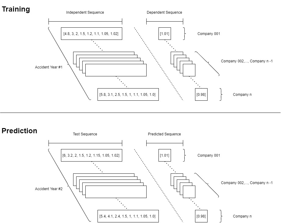
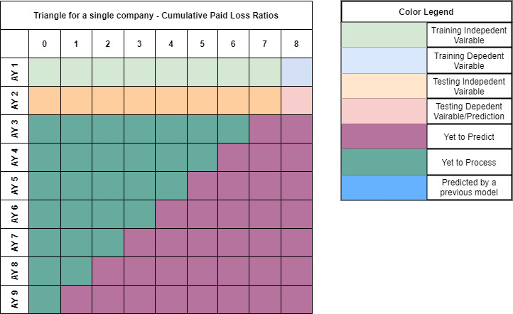
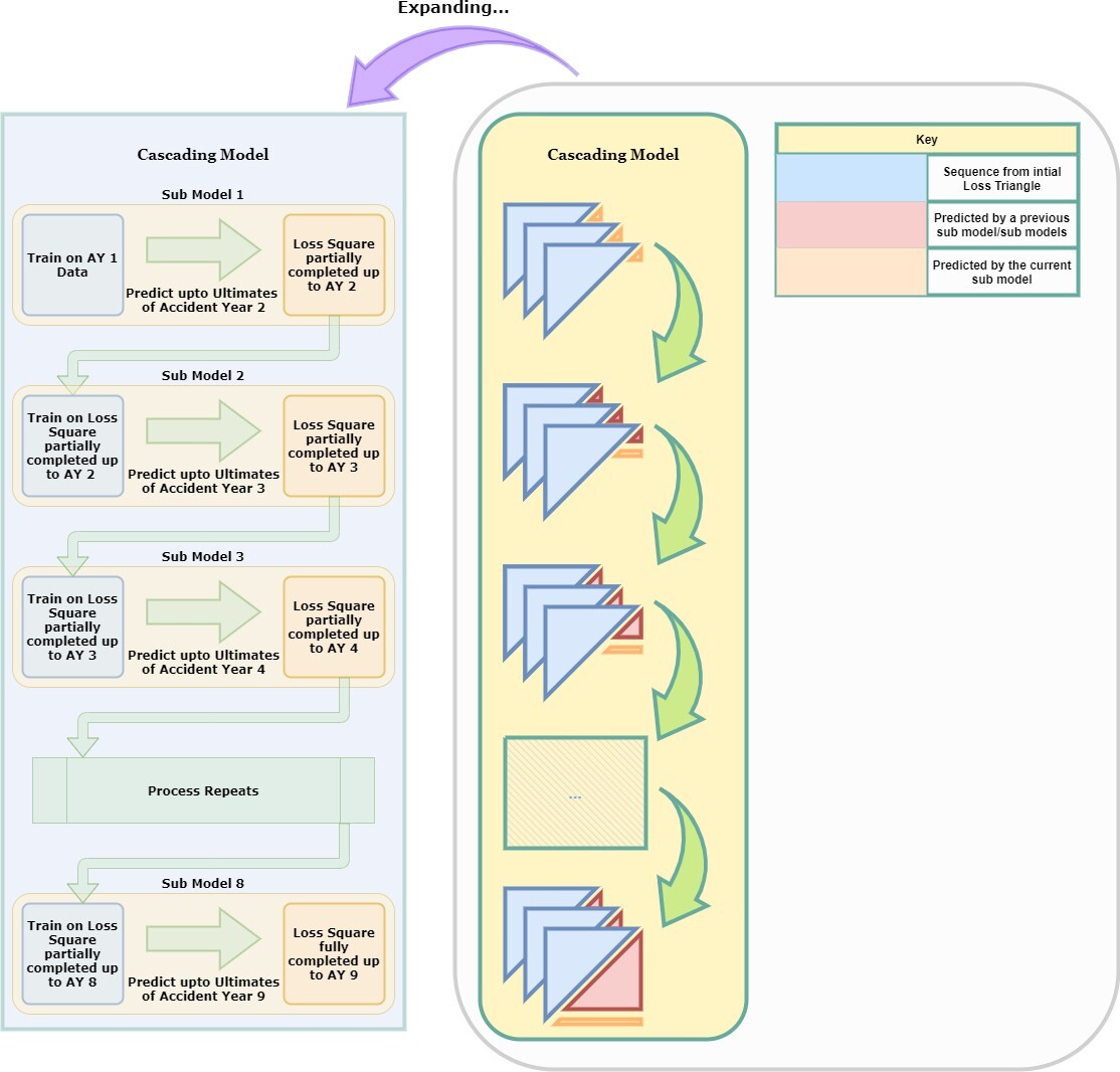
The model of choice for this paper is a composite model which is made of 8 sub-models, making 8 sequence predictions in total. The predictions are recursive in nature with each prediction building on the preceding predictions. Because the loss triangle is an inverted right angle triangle, in order to build a complete square out of the triangle, we need to progressively increase the length of the prediction sequence. We start with the predictions for the first accident year, i.e., the topmost row of the loss triangle. There is nothing to predict in this row. However, we can feed all lag periods barring the last, as a single sequence. This can act as our independent variable. The last lag period can be input into the model as the dependent variable. For both independent and dependent sequences, each stripe of a sequence represents data relates to a single company. For instance, the loss sequence of Company 001 is represented together by the topmost rectangle on the left and the topmost square on the right, in the “Training” portion of Figure 11. It must be noted that this model building process does not aim to complete the loss triangles by completing the diagonals. Instead, we build out each row, from the rows with the most complete sequences (mature data), to those with the least complete sequences (newer data).

Figure 11.Feeding data into a sub-model 1

We can then use the second accident year’s loss sequence, from the first to the penultimate lag as the “test” independent variable. The “Prediction” portion of Figure 11 shows this. Since we want to predict the last lag period’s loss development of the second accident year (this will be our first “true” prediction), we will train our model with the loss sequence from the previous accident year and use that to predict the succeeding accident year’s loss development. For any given company, using the structure shown in Figure 11, we can arrive at a partially completed loss rectangle as shown in Figure 12.

Figure 12.Partially completed loss square, after the predictions made using sub-model 1

After the first sub-model has been made, we use all our previously completed sequence data to make the new dependent and independent loss sequences. We look to see the length of the sequence that we have to predict and then we treat our previous accident years’ data as input. Each accident year is treated as a sample. Figure 13 demonstrates this. In the second sub-model, we have to predict a dependent sequence that is 2 periods in length, and we use the first two accident years of data. For any given company, using the structure shown in Figure 13, we can arrive at a partially completed loss square as shown in Figure 14. Note that the prediction shown in Figure 13 uses predictions made by process shown in the Figure 11.

Figure 13.Feeding data into a sub-model 2

Figure 14.Partially completed loss square, after the predictions made using sub-model 2

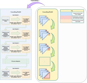
We can generalize the process of building sub-models based on other sub- models, as highlighted in the building of the first sub-model followed by the second sub-model. This can be referred to as “Cascading” (Harej, Gächter, and Jamal 2017). This is illustrated in Figure 15. With reference to Figure 15, the bigger stacked triangles represent the loss triangles of each company in the data set. The first sub-model predicts the ultimate losses of the second accident year of the data set.

Figure 15.General process of cascading

6.1. The Training Data

To successfully implement our deep learning approach, we need so-called training data. This is further explained in Section 2. The training data can be split into two parts: The first part is the independent training sequence while the second part deals with the dependent training variable. To implement the first part, let $S_{r}^{\text{ITRM}}$ denote independent training matrix (ITRM), $S_{r}^{\text{DTRM}}$ denote dependent training matrix (DTRM), $S_{r}^{\text{ITSM}}$ independent test matrix (ITRM), $S_{r}^{\text{POM}}$ denote predicted output matrix (POM), for sub-model $r,$ for $r = 1, 2, \cdots, 8.$ For $R_{k,h,g}$ defined in equation (19) with $k = 0, 1, \cdots, b,$ $h = 0, 1, \cdots, m,$ and $g = 0, 1, \cdots, n,$ $S_{1}^{\text{ITRM}}$ looks at the most mature (or oldest) losses and is given by:

$$S_{1}^{\text {ITRM }}=\left[\begin{array}{ccc} R_{0,0,0} & \cdots & R_{0,0, n-1} \\ \vdots & \vdots & \vdots \\ R_{b, 0,0} & \cdots & R_{b, 0, n-1} \end{array}\right] \tag{20}$$

The second part of the training data is the dependent training matrix (DTRM), $S_{1}^{\text{DTRM}},$ given by

$$S_{1}^{\text {DTRM }}=\left[\begin{array}{c} R_{0,0, n} \\ \vdots \\ R_{b, 0, n} \end{array}\right] \tag{21}$$

The matrix described in 20 represents the oldest losses (losses at accident year 0), from the lag periods 0 through $n-1$ $(n-1=8$ in this case), for each company present in the dataset. The matrix shown in 21 contains the final loss ratio. Together these 2 matrices - $S_{1}^{\text {ITRM }}$ and $S_{1}^{\text {DTRM }},$ form an independent and dependent relationship. This relationship is what is detected by the deep learning algorithm. Once the first sub-model is trained with the above data, we can get the first prediction. We predict with test data. Test data can also be broken into two parts as before; independent and dependent. The independent test data can be shown as:

$$S_{1}^{\operatorname{ITSM}}=\left[\begin{array}{ccc} R_{0,1,0} & \cdots & R_{0,1, n-1} \\ \vdots & \vdots & \vdots \\ R_{b, 1,0} & \cdots & R_{b, 1, n-1} \end{array}\right] \tag{22}$$

The dependent test data or the predicted ultimate loss ratios, are given by the predicted output matrix (POM), $S_{1}^{\text{POM}}$ where

$$S_{1}^{\mathrm{POM}}=\left[\begin{array}{c} R_{0,1, n} \\ \vdots \\ R_{b, 1, n} \end{array}\right] \tag{23}$$

With the test data, in a similar fashion to the training data, we can divide the data into independent and dependent data. In this case, we seek to predict the final loss ratio, for each company in the dataset. Since the Deep Learning algorithm has already been fed with training data, both dependent and independent data - we only need to provide the algorithm independent testing data. With the patterns extracted from the training data using the oldest losses, the sub-model 1 is able to predict the ultimate loss ratio using the loss sequence of the second oldest accident year. Note that the independent data for both training and test data are of the same length, over identical lag periods. The only difference is that with test data, we do not know the dependent value (this is also the first lag which we do not know of, as the second oldest accident year takes one more lag period to fully mature), and therefore this is the matrix we will predict.

The second sub-model therefore processes the two oldest accident years - the two topmost rows of the loss triangle. The second row contains predictions from the previous sub-model. The two rows are split into training data, testing data, and predicted data. The second sub-model can be written as:

$$S_{2}^{\text{ITRM}}= \left[ \begin{array}{c@{}c} \left[\begin{array}{ccc} R_{0,0,0} & \cdots & R_{0,0, n-2} \\ \vdots & \vdots & \vdots \\ R_{b, 0,0} & \cdots & R_{b, 0, n-2}\\ \end{array}\right] & \left[\begin{array}{ccc} R_{0,1,0} & \cdots & R_{0,1, n-2} \\ \vdots & \vdots & \vdots \\ R_{b, 1,0} & \cdots & R_{b, 1, n-2} \end{array} \right] \end{array}\right] \tag{24}$$

S^ITRM is the independent training data matrix. The second part of the training data is the dependent training matrix, S^DTRM, given by

$$S_{2}^{\text{ITRM}}= \left[ \begin{array}{c@{}c} \left[\begin{array}{cc} R_{0,0, n-1} & R_{0,0, n} \\ \vdots & \vdots \\ R_{b, 0, n-1} & R_{b, 0, n} \end{array}\right] & \left[\begin{array}{cc} R_{0,1, n-1} & R_{0,1, n} \\ \vdots & \vdots \\ R_{b, 1, n-1} & R_{b, 1, n} \end{array} \right] \end{array}\right] \tag{25}$$

Once the second sub-model is trained with the above data, we can get the second prediction. Note that in the second sub-model, our goal is to predict the last two lag ratios of the third accident year or third row, for each company. Therefore, our dependent matrix of our training data is two lag periods wide, since we need to train to predict the last two lag periods. This means that the matrix of our independent training data can only be $n-2$ $(n-2=7$ in our case) elements wide. Test data can also be broken into two parts as before; independent and dependent. The independent test data can be shown as:

$$S_{2}^{\operatorname{ITSM}}=\left[\begin{array}{ccc} R_{0,2,0} & \cdots & R_{0,2, n-2} \\ \vdots & \vdots & \vdots \\ R_{b, 2,0} & \cdots & R_{b, 2, n-2} \end{array}\right] \tag{26}$$

Note that the S^ITRM is identical to S^ITSM in width, whilst S^DTRM is identical to S^POM in width. This is done for the same reasons as in the sub-model 1 training - the algorithm knows the nature and dimensions of the independent and dependent relationships of the data for the third accident year. The dependent test data or the predicted ultimate loss ratios can be shown as:

$$S_{2}^{\text {POM }}=\left[\begin{array}{cc} R_{0,2, n-1} & R_{0,2, n} \\ \vdots & \vdots \\ R_{b, 2, n-1} & R_{b, 2, n} \end{array}\right] \tag{27}$$

Following this pattern, the last sub-model, which predicts the ultimates of the last accident year is given as follows:

$$S_8^{\text {ITRM }}=\left[\begin{array}{c} {\left[\begin{array}{c} R_{0,0,0} \\ \vdots \\ R_{b, 0,0} \end{array}\right]} \\ \vdots \\ {\left[\begin{array}{c} R_{0, m-1,0} \\ \vdots \\ R_{b, m-1,0} \end{array}\right]} \end{array}\right], \tag{28}$$

the independent training variable is:

$$S_{8}^{\text {DTRM }}= \left[\begin{array}{ccc} {\left[\begin{array}{ccc} R_{0,0,1} & \cdots & R_{0,0, n}\\ \vdots & \vdots & \vdots \\ R_{b, 0,1} & \cdots & R_{b, 0, n} \end{array}\right]}\\ \vdots \\ {\left[\begin{array}{ccc} R_{0, m-1,1} & \cdots & R_{0, m-1, n} \\ \vdots & \vdots & \vdots \\ R_{b, m-1,1} & \cdots & R_{b, m-1, n} \end{array}\right]} \end{array}\right], \tag{29}$$

the dependent testing data matrix is:

$$S_{8}^{\mathrm{DTRM}}=\left[\begin{array}{c} R_{0, m, 0} \\ \vdots \\ R_{b, m, 0} \end{array}\right] \tag{30}$$

and the predicted output matrix is:

$$S_{8}^{\mathrm{POM}}=\left[\begin{array}{ccc} R_{0, m, 1} & \cdots & R_{0, m, n} \\ \vdots & \vdots & \vdots \\ R_{b, m, 1} & \cdots & R_{b, m, n} \end{array}\right] \tag{31}$$

Once all sub-models have made their predictions, the loss development triangle for each company can be completed and the loss reserves can be estimated.

6.2. Role of Embedding

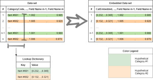
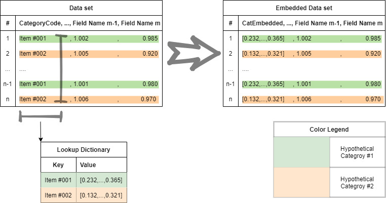
The process highlighted in Section 6.1 is a demonstration of how cascading works with sub-models to create a comprehensive overall model. However, cascading by itself does not help to create an overall modeling process that can predict the loss development of multiple companies at once. As highlighted in Section 6.1, when we input data into the sub-models, we do recognize that the data comes from multiple companies. However, this alone is not enough to ensure that the neural network is aware that it is dealing with parallel sequences of losses from different companies. For that, we need to ensure that we use embedding on each parallel sequence that we input. Embedding is a means to replace original categorical identification data such as categorical names, with vectors (Google 2021). These vectors are deep learning friendly. This process is shown in Figure 16.

Figure 16.Process of Embedding

Embedding is done by first creating a lookup dictionary as shown. Initially, each category is regarded as a key and a subsequent random vector is made for that key in the dictionary. This random vector then replaces each original entry of the categorical name in the data set. By replacing each categorical name with a vector, the substituting vector can be treated like any other variable of the deep learning model. This enables the deep learning algorithm to create a matrix of vectors of length $j,$ where $j$ is the total number of categories in the data, and a width of $w,$ where $w$ is the length of each row, i.e., length of vector representing each embedded category.

7. Sub-Model Architectures

Each sub-model has identical architectures, with the difference being in the size of the input sequences, length of company codes list, the number of bidirectional layers, dense layers, and the width of the output layer. In building a cascading model, the biggest challenge was to build sub-models that progressively increased in the number of parameters in such a way that the respective sub-models did not overfit the data. Hence the reason why the number of bidirectional layers and dense layers gradually increase with the amount of input data. Table 8 gives a brief technical description of the deep learning components used in making each sub-model.

Softplus is not as widely used as some other activation functions such as the Rectified Exponential Linear Unit (RELU). However, on this data set, Softplus tends to perform better than some of the other activation functions, for optimizing using LSTM cells. In terms of the anatomy, Softplus is very similar to RELU with the minor difference of being smoother close to the Input = 0 region. Figure 17 shows these functions. The Scaled Exponential Linear Unit (SELU) activation function is used in the dense layers, with the exception of the output layer. The SELU activation function, much like the Softplus activation, was used due to its performance on the data set. The formulas for each activation function is as follows (Nwankpa et al. 2018):

$$\text { RELU : } \quad f(x)= \begin{cases}0 & \text { if } x<0 \\ x & \text { if } x \geq 0,\end{cases} \tag{32}$$

$$\text{Softplus:} \quad f(x)=\log _{10}\left(\mathrm{e}^{x}+1\right) \quad x \in \mathbb{R}\tag{33}$$

and

$$\begin{aligned} &\text { SELU : }\\ &f(x)= \begin{cases}1.05070098 x & \text { if } x<0 \\ 1.05070098 \times 1.67326324\left(\mathrm{e}^{x}-1\right) & \text { if } x \geq 0\end{cases} \end{aligned}\tag{34}$$

Figure 17.Activation functions used: Softplus (Blue), SELU (Red), RELU (Green)

Since sequence processing involves repeatedly taking derivatives of activation functions, saturation regions in activation functions can lead to vanishing or exploding gradients (Pascanu, Mikolov, and Bengio 2012). The derivatives of Figure 18 show that for values of input (horizontal axis) close to 0 - for any neuron cell, saturation does not occur in Softplus. Perhaps the smooth gradient around 0 in the derivative of Softplus may assist in detecting patterns specific to this data set, hence explaining its better performance. However, further research is needed to confirm this. One similarity between the derivatives of Softplus and SELU is that they do not immediately saturate in the periphery of 0. This could be a potential reason for their good performance on this data set.

Figure 18.Derivatives of activation functions used: Softplus (Blue), SELU (Red), RELU (Green)

The loss function of choice for sequence prediction is mean absolute percentage error (MAPE). This loss function is preferred as the percentage deviation is an equitable measure of deviation, regardless of the normalization used in the sequence (de Myttenaere et al. 2015). In our case, as the data used is ratio data, using the more commonly used mean squared error (MSE) loss function will produce very small errors which may be trickier to optimize. The MAPE loss function is given by:

$$\text { MAPE loss function }=\arg \min _{\hat{y}}\left(\frac{100}{n} \sum_{i=0}^{n}\left(\frac{\hat{y}_{i}-y_{i}}{y_{i}}\right)\right) \tag{35}$$

where $\mathbf{y}=\left(y_{0}, y_{1}, \ldots, y_{n}\right)$ is the vector of observed or actual values and $\hat{\mathbf{y}}=\left(\hat{y}_{0}, \hat{y}_{1}, \ldots, \hat{y}_{n}\right)$ is the vector of predicted or estimated values.

8. Observations - Loss Development Factors and Accident Year/Development Year Interactions

As already established, this model uses loss development factors and consumes data by accident year - to complete each row of the loss triangles of the respective companies. Even so, the business of extracting loss patterns is an endeavor fraught with many dangers. In this section, we aim to consider some of these dangers and also seek to establish the scope of the remedies that we have applied in our approach to minimize these dangers. Loss development patterns can change due to a myriad of reason (Clark and Rangelova 2021):

• Change in the business mix of an insurance company, particularly but not limited to the frequency and severity of claims.
• Changes in the procedures followed - for instance, the process of establishing a case reserve.
• Commutations where the re-insurer transfers its current and future liability from particular ceded contracts back to the original insurer, along with an agreed upon payment. This is a known phenomenon impacting losses from the Schedule P loss triangle - our data source.
• Missing or incomplete data.
• Changes in law and tort reform
• Social inflation causing increases in pay outs.

Data along diagonals, particularly from the later accident years when losses have yet to mature, can become significantly distorted by the above highlighted phenomena. Our model does not aim to tackle any of the above phenomena. Our focus is to merely demonstrate a methodology that can detect and extract loss development patterns. Whilst it is essential that the sources of loss pattern distortions be identified, we feel that doing so in this paper would be a distraction to the fundamental aim of the paper.

De-trending is another important aspect of pre-processing loss development sequences. Whilst knowing the sources of loss distortions can be of immense help, we do not necessarily require this knowledge to de-trend a loss sequence. In our modeling approach, since we consider the loss patterns of all respective companies when making a prediction on any one company’s loss pattern, we partially immunize the model from being too overly sensitive to any idiosyncratic loss trend present in only one company. By considering loss development on a row-by-row basis, we also seek to partially immunize the model from fluctuations present at the diagonal of each loss triangle. Hence our approach to de-trending is embedded in our choice of setting up the model, and also on the inherent virtues of deep learning via recurrent neural networks.

9. The Main Results

Table 9 shows the average deviation of the ultimate loss predictions for each accident year, across all companies, under each method. Deep Learning (DL) is the method implemented in this paper. Chain Ladder is a Python package implementation of loss reserving that is already available for use (Chain Ladder - Reserving in Python 2021). The Chain Ladder Python package has a vast array of functionalities beyond calculating ultimate losses, but for the purposes of this paper, we use it to only calculate ultimate losses.

One important fact to highlight is that under the Chain Ladder package, there is no need to calculate the loss development factors first. Therefore, the loss triangle can start developing from the first accident year. However, under the DL method, since we are working with loss development factors, we have to consume the first two accident years to develop the first ratio, the second two accident years to develop the second ratio and soon. Therefore, in order to create loss data which contain an equal number of lag periods and accident years, we need to omit the first accident year. This is the reason for the AY2 having a prediction of deviation of 0 under the DL method; there is no prediction to be made for AY2.

The prediction deviation is calculated as:

$$\text { Prediction deviation }=\frac{100}{n} \sum_{i=0}^{n}\left|\frac{\hat{y}_{i}-y_{i}}{y_{i}}\right| \tag{36}$$

An example of how the performance deviation is calculated under the Deep Learning (DL) method can be illustrated as follows. Supposing we are interested in the deviation of the $\text{9}^{th}$ lag period of accident year 3 prediction (which is also the Ultimate Loss of AY3).

The Tables 10 and 11 show a pair of sample tables, actual and predicted cumulative paid loss development ratio values respectively, for a sample company. These tables will be used to demonstrate how to calculate performance deviation under the Deep Learning method. The calculations are shown below. Suppose $\left\{\hat{s}_{1}, \ldots, \hat{s}_{i}, \ldots\right\}$ is a sequence of observed or actual values and $\left\{s_{1}, \ldots, s_{i}, \ldots\right\}$ is a sequence of predicted or estimated values and $j$ represents the lag period of evaluation. Then the performance deviation at the $j^{\text{th}}$ lag is:

$$\text { Performance Deviation at Lag } j=\left|\frac{\prod_{i=0}^{j} \hat{s}_{i}-\prod_{i=0}^{j} s_{i}}{\prod_{i=0}^{j} s_{i}}\right| \tag{37}$$

so that the AY3 prediction deviation (at j = 8) becomes

$$\text { AY3 Prediction Deviation }=\left|\frac{\prod_{i=0}^{8} \hat{s}_{i}-\prod_{i=0}^{8} s_{i}}{\prod_{i=0}^{8} s_{i}}\right| \tag{38}$$

Note that for AY3, Table 10 gives $\prod_{i=0}^{8} s_{i}=3.665 \times 2.220 \cdots \times 1.00=13.0707.$ On the other hand, for AY3, Table 11 gives $\prod_{i=0}^{8} \hat{s}_{i}=3.665 \times 2.220 \cdots \times 1.03=13.4628.$

The Tables 12 and 13 show a pair of sample tables, actual and predicted cumulative paid loss values respectively, for a sample company. These tables will be used to demonstrate how to calculate performance deviation under the Chain Ladder method. The calculations are shown below.

$$\begin{aligned} \text { AY3 Prediction Deviation } &= \left|\frac{\hat{y}_{9}-y_{9}}{y_{9}}\right|\\ &=\left|\frac{69.5-69.2}{69.2}\right|\\ &=0.433 \% \text {. } \end{aligned}\tag{39}$$

10. Closing Comments

10.1. Critique of the Inherent Model Limitations

Although the performance metrics shown in Table 9 show us the predictive performance of the overall model, these results do not give us a nuanced insight of the inherent weaknesses of the overall model. The nature of the assumptions which were made in section “Modeling the data,” along with how the loss data develops towards the tails, causes the burden of accuracy of the predictions to weigh heavily on the later sub-models as opposed to the earlier sub-models. This is because the later sub-models have to not only base their predictions on the ever propagating errors of the previous sub-models, but also predict longer sequences with shorter input sequences. This imposes a unique challenge in that the predictions need to account for ever increasing dynamism of data, as the longer into the future, short term trends may not be preserved well (Sánchez-Sánchez, García-González, and Coronell 2019).

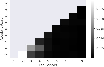
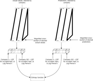
Unlike the beginnings of sequences, the loss development factors at the tails for almost all companies, regardless of the accident year, tend to approach and settle at 1.00. This is an instance of a “concept shift,” where the non-stationary nature of data causes the relationship of extracted features with predicted sequence to change over lag periods (Baier et al. 2020). This means that all sub-models can predict the tail well because the volatility of the tail is comparatively insignificant across all accident years and all companies, when compared to the volatility of loss development factors at the beginnings of the sequences. Under this scenario, the very nature of the ‘cascading’ structure of the overall model presents an inherent limitation to how accurate the predictions of the later accident years can be. In order to study this in detail, the author turned to the entropy package from the scipy library. On the right, the predictions obtained from the overall model are stacked by company. At each lag period, and at each accident year, the loss development factors are extracted. The range of values obtained in this manner can be regarded as a distribution of sorts, unique to this particular lag period and accident year. In a similar manner as explained before, the actual loss development factors at each lag period and each accident year, stacked by company, can be regarded as a distribution. By comparing each pair of distributions, at each accident year - lag period pair, we develop a plot of the entropy at each respective point. The process of how this library is used is shown in Figure 19.

Figure 19.How the entropy analysis works

Figure 20 shows the resulting entropy plot. As anticipated, the earlier lags of later accident years show the most entropy, with a lighter shade showing higher values (lower is better). It should also be noted that the later loss development factors of any accident year are lower in entropy, affirming the inferences made about the nature of the overall model. One plausible reason for this flaw of the overall model may be the limiting characteristics of using a single sequence. Ideally, a second sequence may be able to enable the learning of more patterns. The predicted performances deteriorate for the later accident years and from this plot, we can infer that most of the deterioration occurs at the earlier lag periods and that this error is propagated to the later lag periods as well.

Figure 20.Entropy analysis for the whole model

10.2. Discussion

This project was undertaken with the aim of exploring the possibilities of applications of deep learning in the field of actuarial science. Whilst deep learning may not be as popular in comparison to the more conventional actuarial methods of analysis, there is little doubt of the impact it is due to make in the coming years, especially considering that explosion of the diversity and the vastness of the data that will become ripe for analytics in the future. This project is a minute attempt to contend with a fundamental actuarial problem, in the vast backdrop of the dazzling field of deep learning.

The biggest challenge faced in the context of implementing this project was finding good data that is representative of the real world data. Within this project, data from CAS was used. The nature of deep learning is such that it requires fairly large amounts of data. If larger data sets of comparable type were found, there is more than a fair chance that the predictions could have been of much more superior accuracy.

Another aspect that needs to be highlighted here is the ability of deep learning algorithms to require minimal expert user input. However, this does not mean that we can transcend the limitations of pattern recognition imposed by fundamental laws/theorems of statistics. A case and point of this is how and why we had to normalize loss sequences in a certain manner. The fact that only cumulative paid losses were used also imposed restrictions on the predictive power, since each accident year had only a single channel of a pattern sequence.

Despite these limitations, other than the choice of how to normalize the data as loss development factors, almost all other decisions were related to programming/fundamentals of data science and statistics. The next possible frontier of this project would be the collection of diverse traditional and nontraditional data pertaining to loss reserving, into a single data set, and then building a model that can predict ultimate losses using this diverse portfolio of data.