


1. Introduction
It is no secret that many property and casualty liability lines have seen substantially greater loss development during the past 8–10 years than what was experienced previously. Charts 1 and 2 show the current estimate of ultimate loss and defense and cost containment expense (DCC) divided by reported loss and DCC as of 12 months for commercial auto liability (AL) and general liability (GL) (the combination of other liability–occurrence and product liability–occurrence) for the US domestic industry total. Appendices A and B contain the supporting graphs and tables for AL and GL, respectively. There always has been variability in development, but the development starting around incurred year (IY) 2010 is unprecedented. Loss reserving methods in general assume that future loss development will approximate past loss development. That assumption obviously does not hold in this environment.
2. Data
Annual statement data as of December 31, 2024, was used in this article, specifically Schedule P’s Parts 2 and 4 for loss and DCC data and Part 1 for net earned premium. S&P Global Market Intelligence was used to access this data. Due to the reliance on Schedule P, ultimates are necessarily as of 10 years unless the IY is less mature than that. All ultimates referenced in this article are the booked ultimates. Thus, they will change over time, with later maturities being more accurate than early maturities. Most of this article looks at IYs 2010–2019 to get more reliable booked ultimates and also to mitigate the impact the pandemic had on loss development.
A few notes on nomenclature: The term loss in this article means the sum of loss plus DCC. This article does not address adjusting and other expense. Incurred year is used for the year the loss was incurred, traditionally referred to as accident year. This is done to be consistent with Schedule P and to avoid confusion for nonoccurrence coverages. Also, reported loss means the sum of paid loss and case reserve loss. This is traditionally referred to as incurred loss, but that has a different meaning in an accounting/reporting context. Using reported loss does not mean that report year data is being used. Only IY data is used in this article.
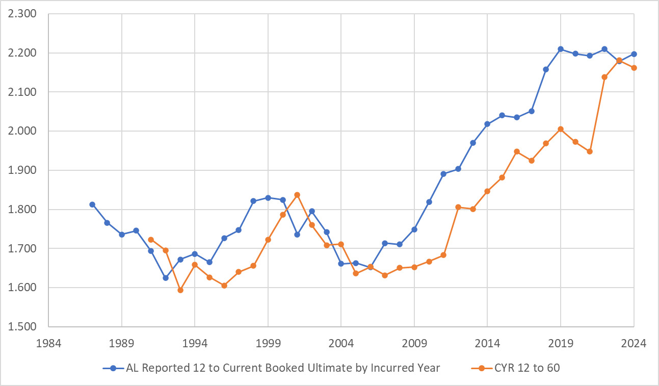
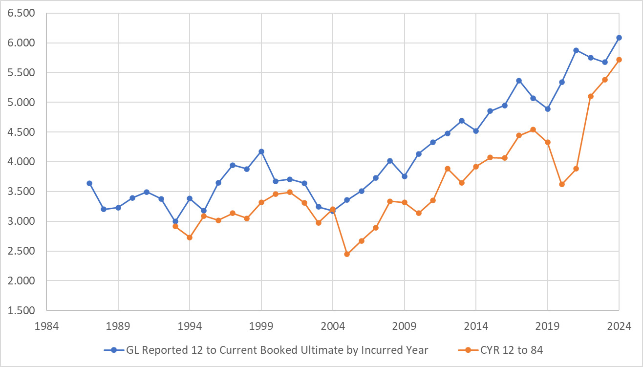
Also shown in Charts 1 and 2 are truncated reported loss cumulative development factors for the calendar year equal to the most recent IY. This article adopts the term calendar-year development factor (CYR), which is used in the article “Social Inflation and Loss Development” (Lynch and Moore 2022). Lynch and Moore describe this as the product of individual age-to-age factors on the diagonal, e.g., the 12–60 CYR equals the product of the link ratios 12–24, 24–36, 36–48, and 48–60. Think of it as the “last 1 of 1” cumulative development factor but taken out to only 60 months for AL and 84 months for general liability (as opposed to taken out to ultimate). As you can see, there appears to be a high level of correlation between the calendar-year reported development factors and the IY 12 to ultimate development. This article leverages this relationship to develop a loss reserve diagnostic that better handles environments with consistently increasing (or decreasing) development.
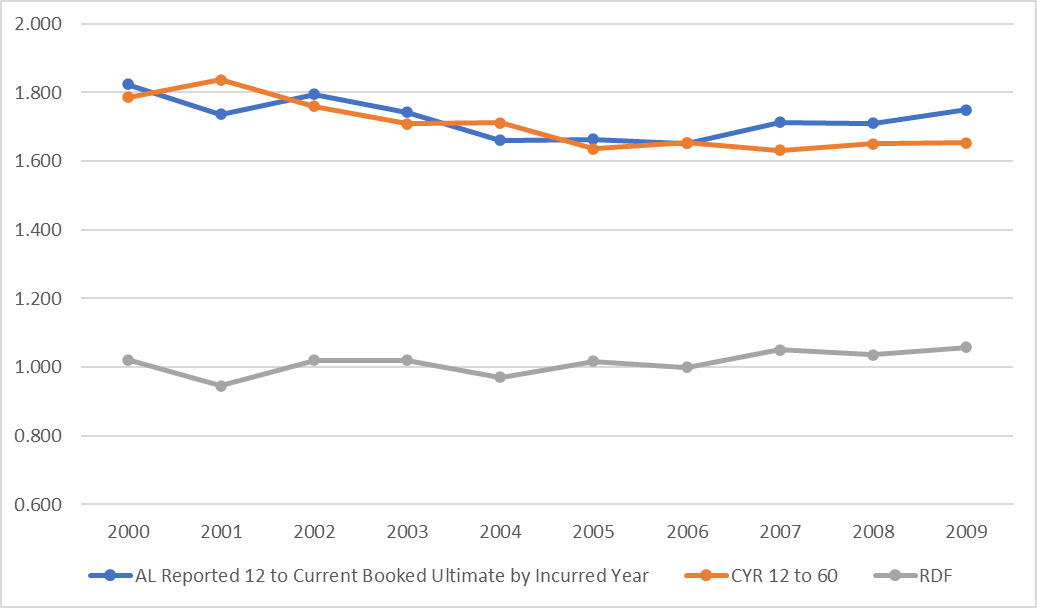
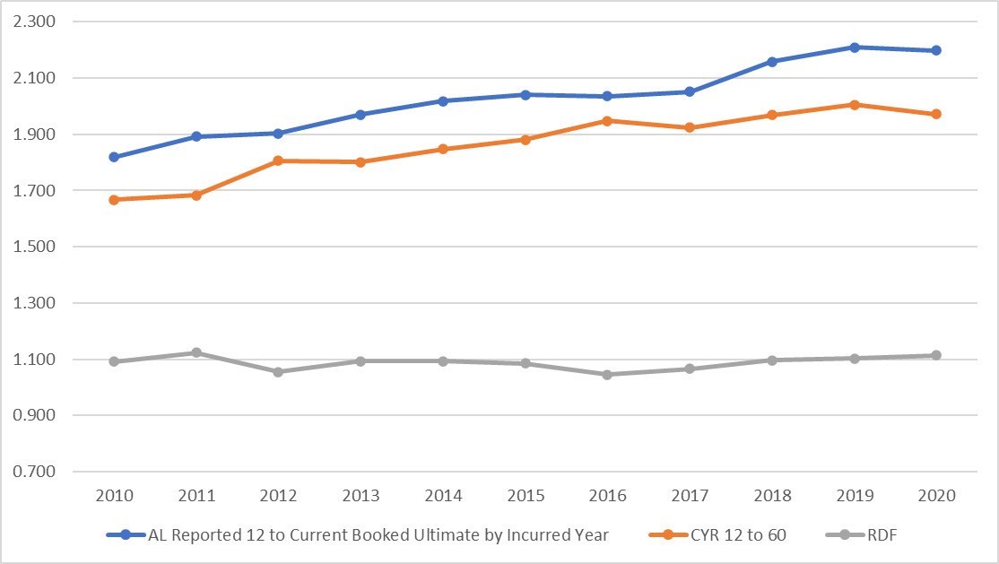
When IY development and CYR development are highly correlated, taking the quotient gives an array that has much less serial correlation and is relatively flat. Chart 3 shows AL IY 12 to ultimate factors, CYR report 12–60 factors, and the resulting quotients for years 2010–2020. While both the IY factors and CYR factor increase pretty steadily, the residual development factor (RDF) line is pretty flat. Indeed the serial correlation for both the IY factors and CYR factors is greater than 90%. The quotient serial correlation is just slightly negative. I define this quotient as the RDF.
3. RDFs
The RDF takes a calendar-year reported development factor to the booked ultimate for the associated IY. Below is a simple example. I assume that losses are fully developed at 48 months. The CYR 12–48 of AL is 1.842 for calendar year 2017, and the reported 12 to ultimate factor for IY 2017 is 2.154 (= 140/65). The RDF is 2.154/1.842 = 1.169. Note that the RDF for an IY will change as it ages if the booked ultimate changes. One could also use paid loss development factors for this, but this article looks only at reported development factors.
In Example 1, the range of RDFs would consist of just two points, 1.048 and 1.169. The current IY RDF (1.101) fits conveniently in that range.
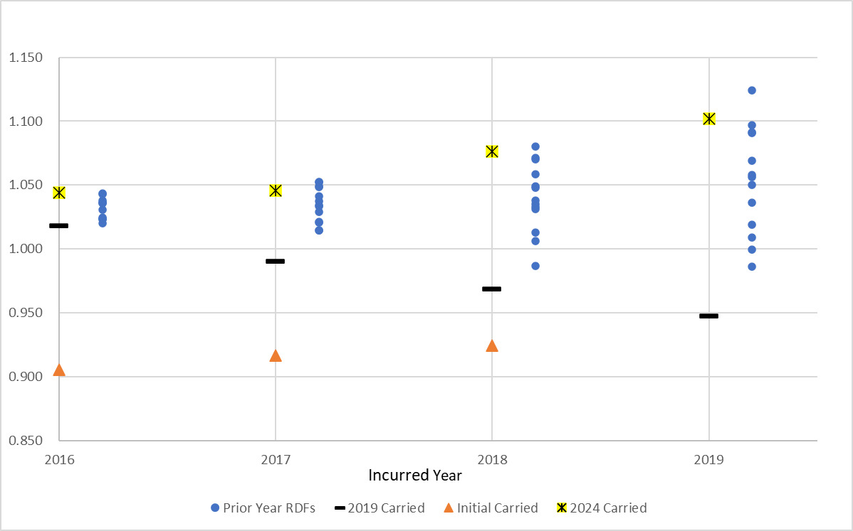
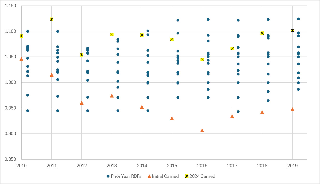
Chart 4 shows IYs 2016–2019 for US domestic industry AL as of the end of 2019. Thus, IY 2016 is as of 48 months, IY 2017 is as of 36 months, and so forth. For each IY, there are 13 prior-year RDFs that constitute a range, the RDF implied from where the IY was initially booked, the RDF booked as of the end of 2019, and the RDF booked as of the end of 2024 for AL.

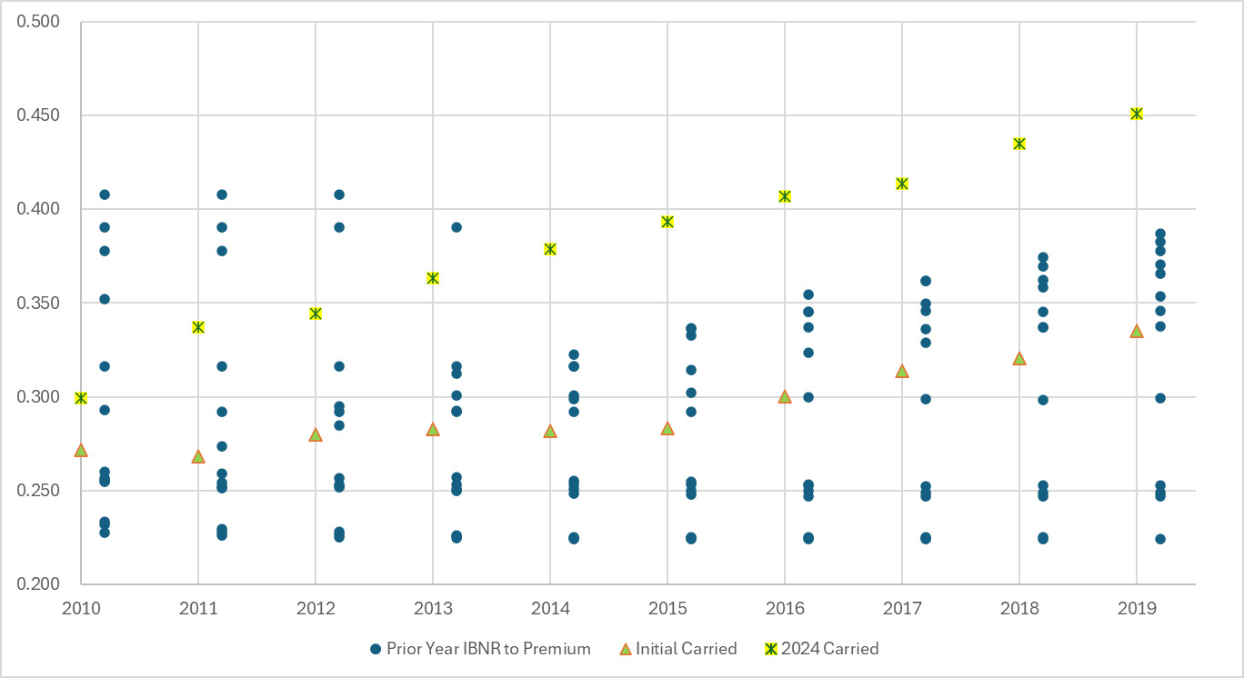
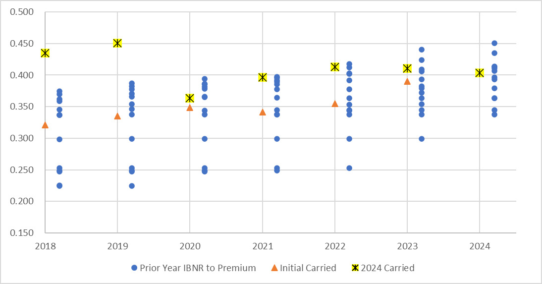
Chart 5 is a version of Chart 4 with 10 IYs (2010–2019), all as of 12 months. The RDFs are all as of the end of the current year, e.g., for 2010, all ultimates used to calculate the RDFs are what were booked at the end of 2010, and so on. Charts 6, 7, and 8 display the same information for the incurred but not reported (IBNR)-to-ultimate diagnostic, IBNR-to-earned premium diagnostic, and last 1 LDF. Table 1 shows the number of current ultimates not in the range for each measure. The RDF diagnostic seems to give a much more robust range across all valuations.
It seems clear that during this time, companies were using some metric along the lines of IBNR-to-ultimate or IBNR-to-premium to guide their initial booking. This resulted in ultimates that were far short of adequate.
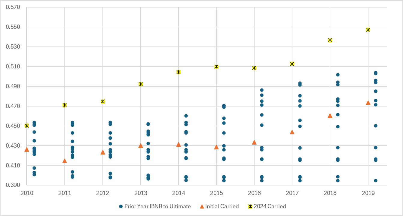

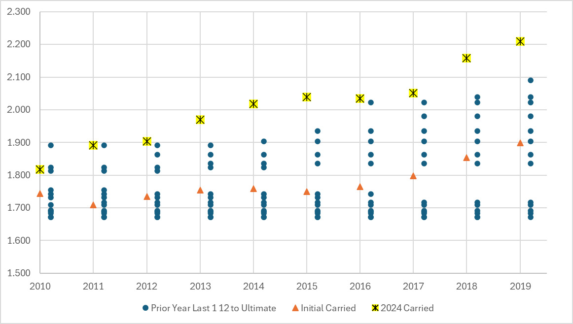
As you can see, the RDF diagnostic much more reliably shows the ultimate result in its range than do traditional diagnostics. It is not surprising that traditional diagnostics don’t capture the ultimate values. If development is consistently increasing, the newer development to ultimate will always be higher than the past. This is not true for the RDF diagnostic.
Is the RDF diagnostic accomplishing this by merely having a wider range? Table 2 shows the width of the range for each diagnostic as a percentage of the current estimate of ultimate (averaged over all 10 IYs). As you can see, the width of the RDF range is comparable to the other diagnostics.
Looking at Charts 5 through 8, it seems evident that the ranges over the IYs exhibit are more stable for the RDF diagnostic. The others show definite changes in the width of the ranges as well as an upward drift. The RDF diagnostic ranges are relatively similar across IYs even in a period of significant change in development factors. This is a roundabout way of saying that RDF ranges are more stationary than other diagnostics; i.e., the statistical properties (e.g., mean, standard deviation) do not change over time as much as other diagnostics. To show this, I calculated the coefficients of variation (= mean/standard deviation) of the means (by IY) and standard deviations (by IY) for the different diagnostics. As you can see in Tables 3 and 4, for AL, the RDF diagnostic has materially lower coefficients of variation for means and lower coefficients of variation for standard deviations. This phenomenon also largely holds in general liability (shown in Appendix B). The greater stationarity of the RDF diagnostic is the main reason it is more robust in periods of persistently changing development.
An attempt to calculate a measure of accuracy for the various diagnostics at 12 months for IYs 2010–2019 is shown in Table 5. For RDFs, IBNR-to-ultimate, and IBNR-to-premium, the average of the midpoint of the range and the mean of the points in the range were used as point estimates. Those estimates were then compared to the current booked figure. For the last 1 LDF method, the indication was used as the point estimate. As you can see in Table 5, the RDF diagnostic is significantly more accurate using this measure than the other traditional diagnostics. For example, the value of –64% shown in the 2010–2019 column and IBNR-to-ultimate row means that the absolute value of the errors by IY are 64% less using the RDF diagnostic than using the IBNR-to-ultimate diagnostic. If the value in the table is positive, it means that the RDF diagnostic has more absolute error than does the other diagnostic. RDFs are not materially more accurate than the last 1 LDF, and in some cases, for other ages and lines, they are materially worse. This is one of the reasons why the RDF method should be a diagnostic, not an indication. It is useful for determining a reasonable range including reasonable high-end or low-end estimates. It can be used to justify indications that fall into its range as reasonable. Simply having indications from various traditional methods does not accomplish this.
4. Other Considerations
Using diagnostics to support reasonability is important for point estimates but maybe more important for reserve ranges. A range of reasonable reserves should have support for both the high and low estimates being reasonable. Just because an indication is the product of a traditional actuarial methodology is not enough. Having a good diagnostic is also helpful when trying to answer senior management questions such as “How bad can this really get?” One can answer this more robustly using RDFs than using other diagnostics.
This issue is even more salient due to the increasing use of sophisticated stochastic models, some using claim-level data, to develop indications. If these models produce indications that are substantially different from traditional indications and diagnostics, how can an outside party gain confidence that the estimates these models produce are reasonable?
The next section attempts to provide answers to anticipated questions about the RDF diagnostic.
4.1. Why are RDFs diagnostics and not indications?
RDFs are stable only at higher levels of volume. RDFs at lower volumes produce very wide ranges as a percentage of ultimate and thus aren’t very useful. Development factors at the coverage level (at which much reserve analysis is rightly performed) are often too volatile for the RDF approach to give meaningful answers. I have used Schedule P line of business because that is what is publicly available, but I would not go much lower than that to apply this measure.
4.2. Aren’t RDFs just tail factors?
Sort of but not really. They are the tail factors that take the CYRs to the booked ultimates for the associated IY. Since the booked amount changes over time, so do the RDFs for an individual IY. They are not selected in an analysis or fit to curves. They are not appropriate to use with other factor averages. RDFs do not specifically measure development after a certain age but rather are the residual development above the calendar-year truncated development. RDFs have both the difference in development at early periods between the calendar year and the IY and the development in the tail. Tail factors and RDFs measure different things and have different intended uses.
4.3. How do RDFs perform at a company level?
No company-level data is in this article. The RDF methodology has been applied to individual companies with success. It probably goes without saying that bigger companies behave better with this diagnostic than do smaller companies. However, there is an adjustment that companies can make. The main issue that occurs when data volume decreases is that the RDF range as a percentage of the ultimate grows and becomes unreasonable. You can simply decrease the width of the range by keeping the mean constant and decreasing the range around the mean of the other points. Alternately, you can use the industry RDF ranges and increase the range of the points around the mean to reflect that an individual company will have a wider range relative to ultimate than the industry total would. How wide the RDF range should be is a matter of judgment. The range sizes for the other diagnostics and the last 1 indications can guide that decision.
4.4. When do RDFs not perform well?
RDFs will not add much value to short-tail lines. They develop so quickly that future development past 18 months or so is typically an issue only with unique situations like late catastrophes or individual large losses.
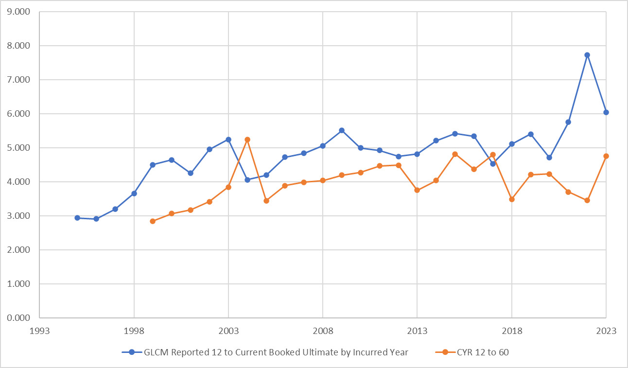
RDFs also will not add much value if the 12 to ultimate factors are not materially correlated with the calendar-year truncated cumulative development factors. General liability claims-made (GLCM) is a good example of this, as shown in Chart 9 (data is through 2023).

The two lines in Chart 9 are basically uncorrelated. If correlation does not exist, using the calendar-year factors doesn’t give you much lift for predicting IY results. As a general rule of thumb, a correlation of at least 40% or so is needed to get material improvement.
4.5. How do RDFs perform when development is neither persistently increasing nor decreasing?
RDFs clearly provide the most benefit versus other diagnostics in environments that have persistently increasing or decreasing development. To test how they perform in an environment that doesn’t display this, I looked at AL for IYs 2000–2009. As Chart 10 shows, development during this period was more stable.

The accuracy measure used earlier in this article shows that IBNR-to-ultimate and last 1 are significantly more accurate than are RDFs. Conversely, RDFs are significantly more accurate during this period than is IBNR-to-premium. As reserving actuaries old enough to remember this period will tell you, the parameter with the most volatility was premium adequacy, not changes in development. Nonetheless, RDFs capture the range of outcomes (as of 12 months) quite successfully. Table 6 shows the comparison.
The improvement isn’t as marked as it is during 2010–2019, but it does score better than the other diagnostics in a period with relatively stable development. Charts 11–14 contain the ranges for all four diagnostics as of 12 months.
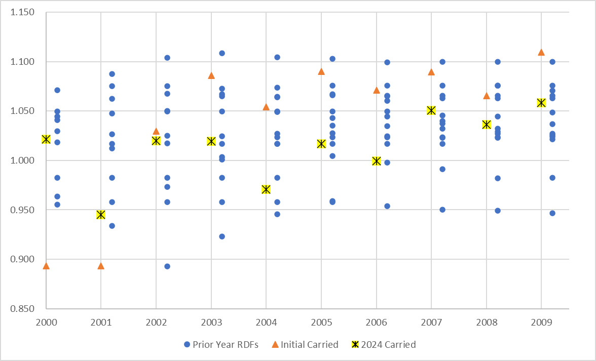
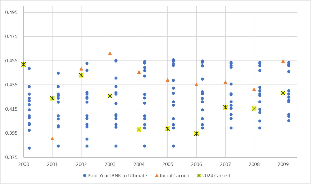
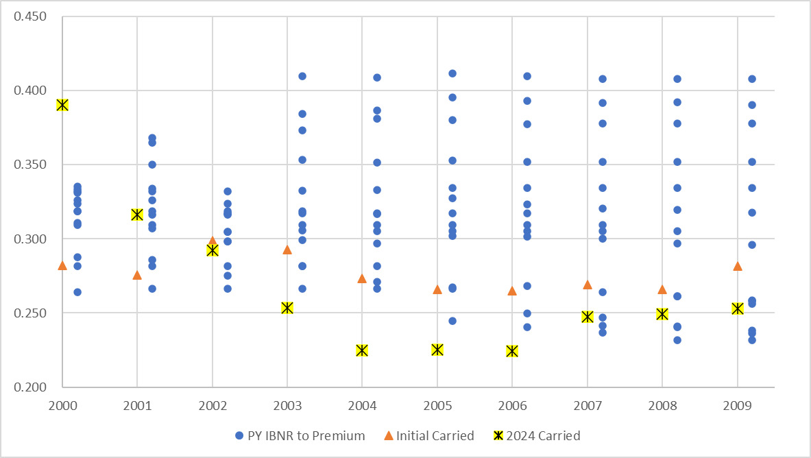
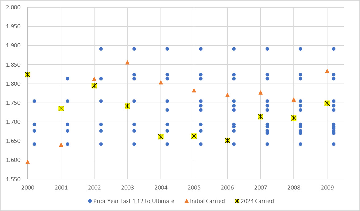
RDFs outperformed the other diagnostics in capturing that range despite the earlier years having less than 13 prior-year results (due to data availability).
As this time period had more stable loss development, RDFs do not exhibit the same improvement in stationarity as was shown in 2010–2019 except compared to the IBNR-to-premium diagnostic.
4.6. How did RDFs do during the pandemic and in postpandemic years?
RDFs performed OK for IYs 2020 and 2021 but did not exhibit the same sort of improvements in accuracy shown in prior years. Part of this may be due to those years not being fully mature yet; i.e., their booked ultimates certainly may change. Having said that, a diagnostic that relies on calendar-year development being correlated with IY development to be most effective probably won’t do well in an environment where claim reporting and settlement are artificially depressed. The booked ultimate for 2022 has increased significantly from the initial booked amount and seems headed to be within the RDF range. Years 2023 and 2024 are already in the RDF range but at the low end. It would not be surprising if those ultimates also moved higher in the RDF range over time. Charts 15–17 display this for RDFs and two other traditional diagnostics for AL.
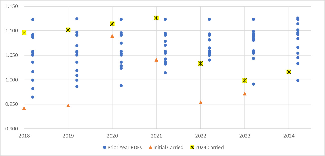
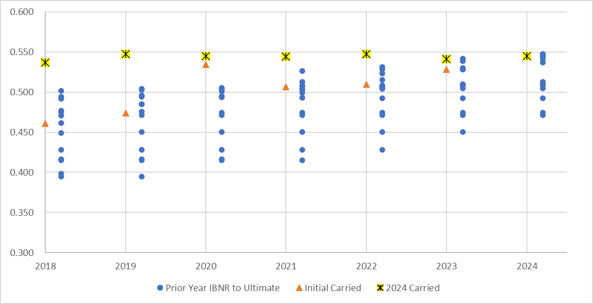

The IBNR-to-premium diagnostic seems to be working best so far, but that may be due to companies relying on that ratio for initial booking and perhaps being slow to change given the uncertainty surrounding development for these years. General liability (graphs shown in Appendix B) shows this phenomenon even more starkly.
5. Conclusion
Traditional loss reserve diagnostics do not work well in periods when loss development shows persistent increases or decreases. RDFs work much better as a diagnostic in these types of environments as long as the age-to-ultimate factors are significantly correlated to the CYRs. RDF ranges more consistently contain the ultimate losses and are more accurate. The RDF ranges are more stationary than the ranges produced by traditional diagnostics.
RDF ranges also provide value during periods of stable development by consistently containing the ultimate values, but they often are not as accurate They can be used to confirm other diagnostic indications during such periods.