GLM for Dummies (and Actuaries)

David R. Clark

1. INTRODUCTION

The introduction of Generalized Linear Models (GLM) in the 1990’s was a revolution for classification ratemaking. GLMs were a leap forward in terms of calculation efficiency and statistical evaluation of the fit of the selected rates. Unfortunately, GLMs have usually been introduced to actuaries (and other audiences) using some advanced statistical distribution theory and model-specific jargon that has been a barrier to widespread understanding. The use of GLMs is mostly the domain of a relatively small group of expert users.

The goal of this paper is to re-introduce GLM with a focus on estimating equations rather than statistical distributions. The estimating equations allow us to view a GLM as a small set of weighted averages. The key idea is to calculate a fitted model such that the weighted average of the fitted loss costs balances to the actual data. This should make the heart of the calculation more intuitive for the non-specialist user of GLM.

The focus on the estimating equations also provides a very straight-forward method for incorporating “prior” information in the analysis to stabilize results when data is sparse, or to limit the change from a prior model.

1.1. Historical Background

The unified model now known as Generalized Linear Models was introduced in 1972 in a paper of that title by Nelder and Wedderburn. They demonstrated that methods for linear regression, logistic regression (for binary outcomes) and Poisson regression (for counts) could all be written in a similar form, with optimal parameters found using the same iteratively reweighted regression algorithm.

Wedderburn generalized the model further with the introduction of “quasi-likelihood” (defined below in section 2.3). Quasi-likelihood behaves like maximum likelihood estimation but with the weaker condition that only mean and variance functions are specified, rather than full distributions. For example, a user can fit a model assuming a constant coefficient of variation (standard deviation divided by mean) without having to specify the distribution as, say, gamma or lognormal.

By coincidence, in the actuarial literature a similar generalization was taking place in credibility theory. Jewell (1974) showed that the linear “N/(N+K)” credibility formula was an exact Bayesian result when the statistical distributions came from the natural exponential family and related conjugate prior – but that the credibility form represented the best linear approximation even if the underlying distribution was not known.

For insurance ratemaking applications, GLMs were adopted in the late 1990’s. Brown (1988) showed the relationship between GLM and the “minimum bias” methods that had been the industry standard. Renshaw (1994) and Mildenhall (1999) gave further mathematical support showing that prior methods from minimum bias were simply particular cases of GLM, and that the iteratively reweighted least squares algorithm gave much greater efficiency in calculating the results.

After the Mildenhall (1999) paper, the use of GLM for ratemaking became the new standard. In addition to the computation efficiency, the ability to show goodness-of-fit statistics and to interpret model coefficients meant that the models were welcomed by insurance departments for rate filing support.

1.2. Objective

The goal of this paper is to provide insight into the working of a GLM. We will focus on the estimating equations that are being solved to find the “best fit” to the historical data. These turn out to have the form of weighted averages of the actual and fitted values, making the interpretation very clear. This also allows for a very straightforward method to incorporate prior information in the form of synthetic data.

1.3. Outline

The remainder of the paper proceeds as follows. Section 2 is the main part of the paper and is outlined as follows

Sect 2.1 Preliminaries: Definition of the Model Components

Sect 2.2 Preliminaries: Univariate Analysis to Understand the Data

Sect 2.3 Key Concept: Estimating Equations

Sect 2.4 Excursus: When is a Poisson not a Poisson?

Sect 2.5 Excursus: What if we get the variance structure wrong?

Sect 2.6 Last Step: Incorporating Prior Information

Section 3 of the paper will summarize some of the conclusions of this outline and suggest future research.

2. GLM for classification ratemaking

We proceed to give a short introduction to the use of GLM in insurance classification ratemaking. This will not cover all of the detailed calculations, or all of the variations on the model that could be used. We will focus only on a basic model and highlight what the GLM is defining as the best fit to the observed data.

To help illustrate the ideas, we borrow the small example from Mildenhall (1999), summarized from data given in McCullagh and Nelder (1989). The example fits a GLM to the severity data for auto liability, using two rating variables (driver age and vehicle use). The data is in Table 1 of the Appendix.

2.1. Preliminaries: Definition of Model Components

The starting point for the model is to define a response or target variable that we are trying to estimate. The response variable is denoted $Y$ and we have a collection of actual observations for that variable $\left\{ y_{i} \right\}$ . For ratemaking, our final objective is to estimate a pure premium (or loss cost), which represents total expected loss relative to an exposure base. In practice we may decompose this into frequency and severity and run separate GLMs on those components.

The response variable is predicted based on a collection of rating variables. In a regression model the predictors take the form of a design matrix, X, with one row of predictors for each observed $y_{i}$ . In classification ratemaking, the predictors are often categorical or “dummy” variables (though they do not have to be), meaning that they are represented as binary (0 or 1) values in the design matrix (see Table 1 of the Appendix for an example). Each row of the design matrix indexed $i$ , corresponds to one observation response variable; each column, indexed $j$ , corresponds to one predictor variable or class.

The main components in our notation are given in the table below.

Figure 2.1.1.

$y_{i}$	Observed values of the response or target variable (e.g., severity, frequency or loss cost).
$w_{i}$	Exposures associated with each $y_{i}$ . For example, when $y_{i}$ is average severity for a class, then $w_{i}$ is the claim count for that average.
$x_{i,j}$	Predictor variables. Typically taking on values of 0 or 1 to represent inclusion in a class $j$ .
$\beta_{j}$	Coefficients fit by the GLM
$\mu_{i}$	Expected or fitted values: $E\left( Y_{i} \right) = \mu_{i}$

The description so far is exactly what you would see in a multiple regression model. GLM expands on the regression approach in two ways.

First, instead of the fitted values being a simple linear combination of the predictor variables, it can be a “link function” of that linear combination. In practice, we do not need to consider all the possible link functions that GLM offers; the “log-link” is generally the approach taken and corresponds to a rating plan in which rating variables are applied multiplicatively.

The log-link function creates the relationship shown in formula (2.1.1).

This relationship assumes rating variables are applied multiplicatively and forces all of the fitted values to be strictly greater than zero (desirable for most insurance applications). It is important to note, that this is not equivalent to a log-linear regression in which we would take logarithms of the observed response variables – in GLM we do not take logarithms of the response variables; we always work with the data in their original units.^[1] This gives two major advantages: first, the model is robust to having some data that is zero or even negative; second, that we do not need to perform an “off-balance” calculation after the fitting is performed.

$E\left(Y_i\right)=\mu_i=\exp \left(\sum_j x_{i, j} \cdot \beta_j\right) \tag{2.1.1}$

The second generalization is for the variance assumption. In regression analysis, there is an assumption that the variance around each observation is equal; in the technical language, this is called homoscedasticity. In practice, we often find that the variance around the observed values is not constant, meaning we observe heteroscedasticity in the data. GLM allows some flexibility to adjust for this by assuming that the variance can be some function of the expected value.

$\operatorname{Var}\left(Y_i\right)=\frac{\phi \cdot V\left(\mu_i\right)}{w_i} \tag{2.1.2}$

In this expression, the parameter $\phi$ (phi) is known as a dispersion parameter. When it is assumed to be constant across the model^[2] it does not affect the GLM fitted values and so is sometimes referred to as a nuisance parameter.

For example, a model with a constant coefficient of variation would have a variance function $V(\mu) = \mu^{2}$ , meaning that the variance is proportional to the squared mean value for each point.

More discussion of the choice of variance function will follow in later sections of this paper.

2.2. Preliminaries: Univariate Analysis to Understand the Data

Before a GLM is run on the full model, it is wise to perform an exploratory step, showing results for each rating variable separately.

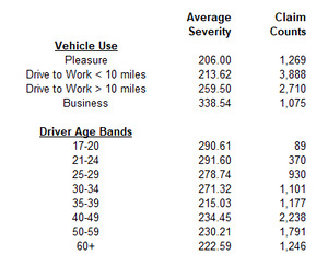
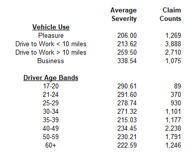
For our simplified example, we look at a GLM for severities of auto liability claims. This severity model has two dimensions, meaning we have two rating variables: driver age and vehicle use. The table below summarizes the average severity for each class within these variables.^[3]

$\text { Average Severity in class } j=\frac{\sum_i y_i \cdot w_i \cdot x_{i, j}}{\sum_i w_i \cdot x_{i, j}} \tag{2.2.1}$

Figure 2.2.1.

This summary of the data is useful because it is a quick way to get an idea of “what our data looks like.” We quickly see, for example, that vehicles used for business generally have higher severity than vehicles used for pleasure. We can also see that the volume of data available for all of the classes varies: the data for the youngest drivers is represented by a much smaller volume of claim counts than the rest of the data.

This univariate analysis is not an optimal way of estimating the values of our rating plan. The distribution of driver ages within any class of vehicle use may not be the same, so we do not want to simply calculate rating relativities from this chart.^[4] The GLM will allow us to evaluate relativities across both dimensions simultaneously.

We will also see that this univariate summary is closely related to the estimating equations in GLM, especially in the “canonical” case (see Section 2.4).

Finally, when reviewing the data, we should keep in mind that the data itself has been prepared for use in the model and the quality of that preparation will also affect the quality of the results. Specifically, we note:

All of the loss data has been adjusted for trend (frequency and/or severity) and brought to an “ultimate” value via loss development.
All of the predictor variables have been identified and are fully populated, with any “missing data” imputed.

In other words, we are assuming that all of the data going into the model is correct and complete. In most cases, getting the data correct and complete is worth more time than some of the nuances of the GLM modeling itself.

For purposes of this paper, we will not address the question of model selection (which rating variables do we want to include), except in passing. In many cases the choice of rating variables will be set based on regulatory and business considerations more than statistical or machine learning criteria. This paper will focus only on how the GLM estimates the best parameters for the selected rating factors.

2.3. Key Concept: Estimating Equations

In this section we will show the derivation of the estimating equations used in the GLM. The estimating equations are (like the normal equations in regression) what is being solved to find the “best” set of coefficients. The derivation itself is not needed to appreciate the result. The mathematics serve – to borrow a phrase from Wittgenstein – as “a ladder to throw away after we have climbed up.”

The quantity that we are maximizing in the GLM is known as a quasi-likelihood (QLL) function (see Wedderburn (1974), McCullagh (1983)). This behaves like a log-likelihood function in traditional maximum likelihood estimation (MLE), but it is more general in that it only requires knowledge of the variance structure.

$\text { Quasi Likelihood }=Q L L=\sum_i w_i \int_{y_i}^{\mu_i} \frac{y_i-t}{\phi \cdot V(t)} d t \tag{2.3.1}$

This definition looks a bit intimidating because of the integral. But when we want to find the model parameters to maximize it, we are not interested in the QLL itself, but only the derivatives with respect to the parameters. This is where the simplification comes in. When the log-link is used, the derivative is shown in (2.3.2).

$\frac{\partial Q L L}{\partial \beta_j}=\sum_i w_i \cdot \frac{y_i-\mu_i}{\phi \cdot V\left(\mu_i\right)} \cdot \mu_i \cdot x_{i, j} \quad \forall j \tag{2.3.2}$

Setting the derivative equal to zero for each parameter $\beta_{j}$ produces the set of estimating equations that are the condition to be met for an optimal fit to the data.

$\small{ \sum_i y_i \cdot w_i \cdot\left(\frac{\mu_i}{V\left(\mu_i\right)}\right) \cdot x_{i, j}=\sum_i \mu_i \cdot w_i \cdot\left(\frac{\mu_i}{V\left(\mu_i\right)}\right) \cdot x_{i, j} \quad \forall j \tag{2.3.3} }$

From formula (2.3.3) we see that the fitted values $\mu_{i}$ will “balance” to the actual data across every rating variable (every column of the design matrix $\mathbf{X}$ ), under the weights specified by the variance structure. GLM can be viewed as a sophisticated weighted-average calculation.

The estimating equation also implies a re-weighted average severity across each predictor variable. Formula (2.3.4) shows how the univariate analysis would change with the adjusted weights. The fitted GLM will balance to this re-weighted average severity across each rating variable.

$\small{ \text { Reweighed Severity in class } j=\frac{\sum_i y_i \cdot w_i \cdot\left(\frac{\mu_i}{V\left(\mu_i\right)}\right) \cdot x_{i, j}}{\sum_i w_i \cdot\left(\frac{\mu_i}{V\left(\mu_i\right)}\right) \cdot x_{i, j}} \tag{2.3.4} }$

The table below illustrates the estimating equations for several choices of the variance function. Once we have this table, we never have to think about quasi-likelihood again.

Figure 2.3.1.

$\mathbf{Var}\left( \mathbf{Y} \right)$	Related Distribution	Estimating Equations (Log-Link)
$\phi$	Normal	$\sum_{}^{}{{y_{i} \cdot w}_{i} \cdot \left( \mu_{i} \right) \cdot x_{i,j}} = \ \sum_{}^{}{{\mu_{i} \cdot w}_{i} \cdot \left( \mu_{i} \right) \cdot x_{i,j}}$
$\phi \cdot \mu$	Poisson	$\sum_{}^{}{{y_{i} \cdot w}_{i} \cdot x_{i,j}} = \ \sum_{}^{}{{\mu_{i} \cdot w}_{i} \cdot x_{i,j}}$
$\phi \cdot \mu^{2}$	Gamma	$\sum_{}^{}{{y_{i} \cdot w}_{i} \cdot \left( \mu_{i}^{- 1} \right) \cdot x_{i,j}} = \ \sum_{}^{}{{\mu_{i} \cdot w}_{i} \cdot \left( \mu_{i}^{- 1} \right) \cdot x_{i,j}}$
$\phi \cdot \mu^{3}$	Inverse Gaussian	$\sum_{}^{}{{y_{i} \cdot w}_{i} \cdot \left( \mu_{i}^{- 2} \right) \cdot x_{i,j}} = \ \sum_{}^{}{{\mu_{i} \cdot w}_{i} \cdot \left( \mu_{i}^{- 2} \right) \cdot x_{i,j}}$
$\phi \cdot \mu^{p}$	Tweedie	$\sum_{}^{}{{y_{i} \cdot w}_{i} \cdot \left( \mu_{i}^{1 - p} \right) \cdot x_{i,j}} = \ \sum_{}^{}{{\mu_{i} \cdot w}_{i} \cdot \left( \mu_{i}^{1 - p} \right) \cdot x_{i,j}}$
$\phi \cdot \left( \mu + \frac{1}{k} \cdot \mu^{2} \right)$	Negative Binomial	$\sum_{}^{}{{y_{i} \cdot w}_{i} \cdot \left( \frac{k}{k + \mu_{i}} \right) \cdot x_{i,j}} = \ \sum_{}^{}{{\mu_{i} \cdot w}_{i} \cdot \left( \frac{k}{k + \mu_{i}} \right) \cdot x_{i,j}}$
$\phi \cdot \left( \mu + \frac{1}{k} \cdot \mu^{3} \right)$	Poisson-Inverse Gaussian	$\sum_{}^{}{{y_{i} \cdot w}_{i} \cdot \left( \frac{k}{k + \mu_{i}^{2}} \right) \cdot x_{i,j}} = \ \sum_{}^{}{{\mu_{i} \cdot w}_{i} \cdot \left( \frac{k}{k + \mu_{i}^{2}} \right) \cdot x_{i,j}}$
$\phi \cdot exp\left( \frac{1}{k} \cdot \mu \right)$	???	$\sum_{}^{}{{y_{i} \cdot w}_{i} \cdot \left( \mu_{i} \cdot e^{- \mu_{i}/k} \right) \cdot x_{i,j}} = \ \sum_{}^{}{{\mu_{i} \cdot w}_{i} \cdot \left( \mu_{i} \cdot e^{- \mu_{i}/k} \right) \cdot x_{i,j}}$

But here an additional word is needed about the “related distribution” associated with each of these variance structures. These labels come from special cases.^[5]

The original Nelder & Wedderburn paper in 1972 noted that several existing regression models could be solved using the same algorithm. Part of the insight was that the various distributions (Gaussian, Bernoulli, Poisson) could all be written in a natural exponential family form.

$f(y \mid \theta, \phi)=\exp ((\theta \cdot y+b(\theta)) \cdot a(\phi)+c(y, \phi)) \tag{2.3.5}$

This form is not the way most of the distributions are presented in introductory statistics books, but it is very convenient when solving for the maximum likelihood estimate. As with quasi-likelihood, the optimal parameters are found by setting the derivatives equal to zero . The derivative of the logarithm of the density function in (2.3.5) is shown below.^[6]

$\frac{\partial \sum \ln \left(f\left(y_i \mid \theta, \phi\right)\right)}{\partial \theta}=\sum\left(y_i+\frac{\partial b(\theta)}{\partial \theta}\right) \cdot a(\phi)=0 \tag{2.3.6}$

This form makes the estimating equations linear in terms of the response variable.^[7] This is the same as the quasi-likelihood derivation above, meaning that the examples from these specific distributions are special cases of the more general form.

This generalization is critical: it means that we can use the variance structure borrowed from discrete distributions (Poisson or Negative Binomial) even for continuous random variables. We can also use the “Tweedie” structure with variance parameter $0 < p < 1$ , even though the Tweedie is really only defined for $1 < p < 2$ .

GLM is best thought of in terms of variance structure even though we use the language of distributions.

The last comment related to the mathematical structure of GLM is that the second derivatives of the quasi-likelihood function are almost as easy to calculate as the first derivatives. This provides the tools for a very efficient algorithm to be used to iteratively solve for the model parameters. The algorithm is iteratively reweighted least squares (IRLS), which is related to the Newton-Raphson algorithm. In most cases, best fit parameters can be found in fewer than 10 iterations of the routine.

2.4. Excursus: When is a Poisson not a Poisson?

The use of the “Poisson” name in GLM is a blessing and a curse for actuaries. Actuaries are trained to think in terms of statistical distributions, and we are very familiar with the Poisson distribution. In practice, however, the Poisson distribution itself is generally not a good model for insurance phenomenon and zero-modified or over-dispersed (e.g., negative binomial) frequency distributions are more realistic.

But here is the good news: GLM does not need to assume that loss counts come from a Poisson distribution. We are only using the assumption that the variance is proportional to the mean value. We do not need to assume that the variance equals the mean. We do not even need to assume that the distribution is defined on the non-negative integers; values can be non-integers and even include some negative values (so long as the average is positive).

We might say there is something fishy about using the Poisson label.

If we know that the data comes from a Poisson distribution then $Var(Y) = E(Y)$ ; but if we only know that $Var(Y) = \phi \cdot E(Y)$ , (even if $\phi = 1$ ) then it is not necessary to assume that the data comes from a Poisson distribution.

The key advantage in using this variance structure with the log-link GLM is that the logarithm is the “canonical” link function. In practice what this means is that estimating equations are simplified and do not include the extra weighting function. The estimating equation turns out to be equivalent to the Bailey “minimum bias” criteria and means that the univariate summaries on the fitted values will look exactly like the univariate summaries of the original data.

2.5. Excursus: What if we get the variance structure wrong?

The GLM framework allows for a wide choice of variance functions. This gives a way to reflect the heteroscedasticity in the actual loss data. While the model is not overly sensitive to changes in the variance function, it is still important to validate the choice we make.

We first estimate the dispersion parameter. While there are alternatives to how this can be estimated, the easiest is given in formula (2.5.1).

$\hat{\phi}=\frac{1}{n-p} \sum w_i \cdot \frac{\left(y_i-\mu_i\right)^2}{V\left(\mu_i\right)} \quad \begin{aligned} & n=\# \text{data points} \\ & p=\# \text{parameters} \end{aligned} \tag{2.5.1}$

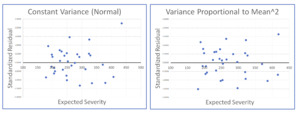
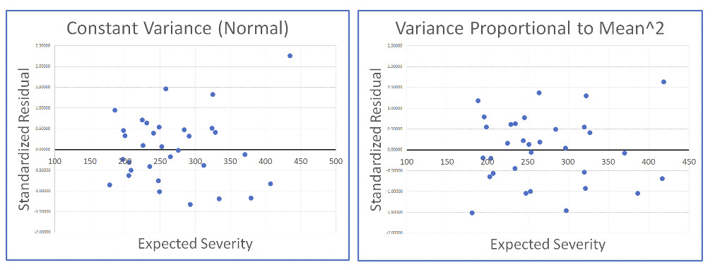
The standardized residual^[8] corresponding to each observation is given in formula (2.5.2). If our assumption about the variance structure is correct, then we should see in the residual plot roughly the same spread of points across the range of fitted severities.

$\text { Standardized Residual }_i=\left(y_i-\mu_i\right) \cdot\left(\frac{w_i}{\widehat{\phi} \cdot V\left(\mu_i\right)}\right)^{1 / 2} \tag{2.5.2}$

Using the auto severity example, we can look at the residual plots for two very different variance structures. On the left we have the residuals assuming variance is constant for all severities (Normal); on the right are the residuals assuming variance is proportional to the square of the expected severity (Gamma). While there is some evidence of heteroscedasticity in the graph on the left, it is not entirely clear that one assumption is superior to the other.

Figure 2.5.1.

Because the heteroscedasticity of the residuals may be hard to use to identify the “correct” variance structure, the practical approach is to select the variance structure judgmentally when the model is set up and then only use the residuals to validate, or to change the variance assumption if something is clearly wrong.

In his book, “Multiple Regression: A Primer,” Paul Allison says, “My own experience with heteroscedasticity is that it has to be pretty severe before it leads to serious bias in the standard errors. Although it is certainly worth checking, I wouldn’t get overly anxious about it.”

2.6. Incorporating Prior Information

A practical problem in classification ratemaking is that it is desirable to have a detailed rating plan that can capture even subtle differences between risks. At the same time, the available data may be more limited, with some classes under-represented in the experience period or even missing altogether. This is the problem of over-fitting to the data – chasing noise rather than getting the true best estimate.

An easy way to stabilize^[9] the result of the model, and avoid chasing the noise, is to incorporate a credibility procedure using synthetic data as prior information. This approach has a long history in statistical modeling as described in the papers by Huang et al. (2020) and Greenland (2006, 2007).

The concept of data priors also connects closely with Bayesian credibility ideas. Jewell (1974) showed that linear credibility was exact in the case of exponential family distributions with their conjugate priors. In those cases, the information from the conjugate prior can be treated as prior data directly.

Our choice for the prior information might come from one of three sources:

A simpler model (e.g., a model with fewer classes) on the same data set
Insurance industry data (e.g., ISO, NCCI)
Prior version of the company’s rating plan (e.g., rates currently in place, after appropriate adjustment for trend^[10])

The use of a simpler model on the data was suggested in Huang et al. (2020) with reference to past studies using occupancy data – an example that may resonate with actuaries pricing workers’ compensation risks. The problem was that the detailed data included too many specific job classifications (current NAICS codes include more than 1,000 classes). However, the detailed job classes could be grouped into 20 broader categories. A model is run first on the data with the 20 broader categories as predictors; the results of that model could then be blended with the more detailed data to stabilize the final model.

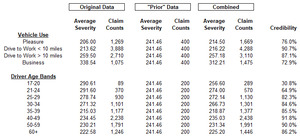
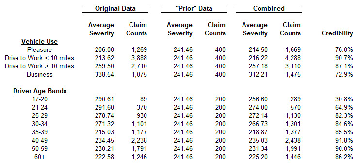
To illustrate this with our auto severity example, we can use as a simpler model the assumption that every class has the same severity. For every age band / vehicle use combination we add a few additional losses assigned this average amount. The GLM is then run on the enhanced data set (what Huang calls the “working model”). Table 2 of the Appendix shows this calculation. The univariate analysis on the data shows how this use of synthetic data is a simple credibility weighting.

Figure 2.6.1.

The question then turns from how to implement credibility to how much weight to assign to the prior data. The short answer is that we want to include “just enough” prior information to stabilize the outcome. Huang refers to this insightfully as a “catalytic prior” – that is, we want enough to make the result work.

For the insurance application, it is best to think of the prior as being last year’s rating plan. Our goal is to fit a new rating plan to the current data but to constrain the results to keep the change from the old rating plan within a selected tolerance.

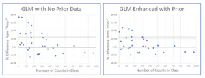
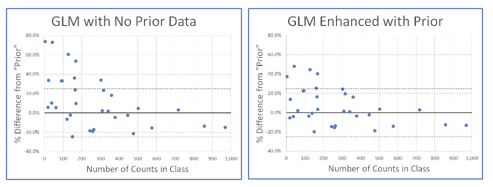
The graphs below show the basic idea. Each point represents one age band / vehicle use combination or class. The horizontal axis is how many claims we have in the data for each of these classes. The vertical axis is the percent change from the “prior” model (assuming in the past each class had the same severity). On the left, the percent changes are based on a model with no prior information included; the percent changes for classes with few claims can be very large. On the right is the result from the GLM including 50 synthetic claims into each class; the percent changes can be reduced greatly, though the classes with a high volume of claims in the original data are minimally affected.

This type of analysis can be easily implemented so that the change in a model using updated data can be constrained to be within a set tolerance.

Figure 2.6.2.

3. RESULTS AND DISCUSSION

This paper is intended to help explain the basic concepts underlying GLM, while avoiding some of the technical language that is a hurdle for someone seeing it for the first time.

The example used was on auto severity, but frequency or loss cost response variables work in the same way; we just change the weights $w_{i}$ from claim counts to some exposure base (perhaps policy counts). The example uses categorical “dummy” variables of 0 or 1 in the design matrix, but these can also be changed to continuous variables with no change to the mathematical calculations.

3.1. Key Concepts for Actuaries

Two key concepts in GLM may cause some confusion to actuaries given our background and training.

First, the introduction of the log-link is a possible confusion because an actuary may immediately think of log-linear regression. Actuaries often work with log-linear regression in problems such as estimation of severity inflation trend: the regression analysis starts by taking the logarithm of the historical severity numbers. The GLM log-link is different because we never take the logarithm of the empirical data but are always working with it in its original units. Dollars stay as dollars, and not log(dollars).

Second, actuaries are trained to think in terms of statistical distributions, but GLM is only working with variance functions - even though distribution names are retained as labels. When an actuary sees something labelled “Poisson,” they will assume it only works for discrete distributions. The “Poisson” model in GLM is much more flexible.

In fact, you do not need to know anything about the exponential family of distributions in order to understand GLM.

3.2. Future Research

GLM is a very flexible tool and well-suited for the classification ratemaking application. It is also easier to implement and understand than may appear at first. Many extensions beyond the basic GLM are possible and worth further research. Two items are of special note.

First, this paper has shown how prior information can be included in the model in the form of synthetic data. This method is not yet in widespread use and further research into how the prior information can best improve predictive accuracy is worthwhile.

Second, a key assumption in GLM (as with linear regression) is that all the observed data points are statistically independent. This is unlikely to be true in reality, but the assumption is used when estimating significance tests on the fitted parameters. If the independence assumption does not hold, then we may reach incorrect conclusions on which rating variables to keep in the model. Correlation may be imposed by the analyst in trending and developing historical data. It could also come from external sources; the recent covid pandemic and subsequent supply-chain-related inflation spike provide a dramatic example of external factors. More research would be helpful into how to reflect this uncertainty and correlation into the standard errors.

4. CONCLUSIONS

GLM is a very powerful tool, especially as the “log-link” allows us to fit models with strictly positive expected values. The GLM allows us to do this without transforming the original data, so that the fitted model will always balance to the original data under specified weights.

Most important for the pricing actuary is that a GLM can be viewed as a weighted average model, where the weighted average of the fitted model balances to the weighted average of the actual data. The “actual” data is often adjusted for trend and development. This means that the priority should be getting the trend and development correct.

Recognizing the importance of the estimating equations as weighted averages also leads to a natural method for incorporating prior information.

Acknowledgment

The author gratefully acknowledges the helpful comments from Yun Bai, Le (Louis) Deng, Lulu (Lawrence) Ji, Clifton Lancaster, Ulrich Riegel, Ira Robbin, Bradley Sevcik, and Janet Wesner in early drafts of this paper. All errors in the paper are solely the responsibility of the author.

Abbreviations used in the paper

GLM, generalized linear model	IRLS, iteratively reweighted least squares
MLE, maximum likelihood estimation	QLL, quasi-likelihood

Biography of the Author

David R Clark, FCAS is a senior actuary with Munich Re America Services, working in the Pricing and Underwriting area. He is a frequent contributor to CAS seminars and call paper programs.