The Variability and Tail Behavior of Compound Climatic Normal Conditions

Abbreviations and notations

DH — Dry-hot
WW — Wet-warm
EDC — Extreme dry-cold
SDH — Strong dry-hot
SN — Skew-normal (SN)
KS — Kolmogorov Smirnov
$w_{t}$ — white noise
A — Amplitude
f — Frequency
t — Time (in months)
$\varphi$ — Phase
T — Periodic time

1.0. Introduction

Extreme climate events have a low probability of occurring but a potentially large immediate adverse effect on communities, nevertheless, little shifts in the normal climatic states could also lead to loss of lives and livelihoods over a long period, for example due to coastal erosion and desertification. van der Wiel and Bintanja (2021) specifically attributed the frequency of climate extremes to the shifts that occur in both mean climate and climate variability. They studied temperature and precipitation independently and their work can be seen to align with that of Lewis and King (2016) who also examined, from the perspective of distributional shifts and shape changes, the impact of mean temperatures on temperature extremes. Considering the joint climatic variables of mean temperature and rainfall, Mesbahzadeh et al. (2019) studied the interdependence of precipitation and temperature in Iran by applying scenarios of the fifth Intergovernmental Panel on Climate Change (IPCC) assessment report. The Frank and Gaussian copulas were the best fit for the different scenarios. Rana, Moradkhani, and Qin (2016) also used copulas to model the joint distribution based on the data generated at Portland State University. The authors then estimated future trends, noting that dry season generally indicates a higher positive change in precipitation than in temperature. Other similar studies employing copulas include Ayantobo, Wei, and Wang (2021) and Tencer, Weaver, and Zwiers (2014)for the cases of mainland China and Canada, respectively.

The compounded events resulting from the joint interaction of precipitation and temperature have severe impacts on agriculture, economy and public health as highlighted by Hao et al. (2020). Focusing on compound dry-hot event, the authors studied the influence that El Niño–Southern Oscillation (ENSO) has on temperature and precipitation by investigating the joint distribution of temperature, precipitation and the ENSO indicator in selected parts of Canada, South America, Asia, Africa and Australia. Their conclusions indicated that ENSO has a significant impact on the risk of compound dry and hot events in the regions of choice. A number of previous studies (Miao et al. 2016; Zscheischler et al. 2020; Zscheischler and Fischer 2020; Zhang et al. 2022; Bevacqua et al. 2021) have also examined the joint probabilistic characteristics and tendencies that are exhibited by bivariate and even trivariate precipitation and temperature indices across different countries. In particular, Zscheischler et al. (2020) categorized compound event types into four themes namely, preconditioned, multivariate, temporally compounding, and spatially compounding events. Bevacqua et al. (2021) further illustrated how these four types can be studied pragmatically using case studies of different compound event types in Australia, Portugal, France and Germany.

It has generally been noted that research on the analysis, quantification and prediction of compound events is still at its infancy stage and most of the studies in literature address compound events in countries located in the Global North -Germany, Spain, France, USA and the UK to mention a few. However, to the best of the author’s knowledge, there are no studies that have addressed how these compound climatic risks can be incorporated into the general risk management framework. This is where the actuarial community has a major role to play. Research on a developing model, the Actuaries Climate Risk Index (ACRI), is being carried out. It aims to measure/quantify the loss-dollar risk posed by climate change in US and Canada after controlling for factors such as inflation, exposure, region and seasonality (https://actuariesclimateindex.org/home/). India, under the direction of the National Institute of Disaster Management and GIZ, has also set up a framework for climate risk management to address loss and damage that are driven by context-specific needs in the country (Mechler et al. 2019). They highlighted the insufficient methodologies that exist in assessing and managing long-term, slow-onset climate hazards in contrast to those available for short-term events (mostly extreme events). Their framework incorporated local techniques such as focus groups at the community level in a bid to better understand and manage the climate risks. Although these research works are indicative of the significant positive progress experienced within the field of climate risk management, the risk posed by compounding climatic events has not yet been accounted for in both cases of ACRI and the Indian framework. This critical gap limits the models’ usage in accurately estimating the hazardous events/compound costs that are driven by the compound interactions of climatic variables.

The lack of research in compound climate events is even more glaring in the case of India where there are extremely fewer studies (Guntu and Agarwal 2021; Das, Manikanta, and Umamahesh 2022), notwithstanding the IPCC report that predicts more high- impact compound extremes for India (Nandi 2021). Worse still, is the case of African countries, a region where the compounding climatic events get to interact with already existing deep-rooted socio-economic problems. The available research studies include Weber et al. (2020), Camara, Diba, and Diedhiou (2022), Chukwudum and Saralees (2022) and Zscheischler and Lehner (2022). This paper builds on the research work of Chukwudum and Saralees (2022) by contributing to literature in two ways. Firstly, the tail behaviour of the joint climatic variables of mean temperature and rainfall in different African (Nigeria, Ethiopia, South Africa) and Asian (India) countries is studied. These are regions that have received very little attention in terms of compound climate studies. The compound climatic types to be evaluated are dry-hot, extreme dry-cold and wet-warm environmental conditions. Attention is paid to modelling the climate variability of the strong dry-hot condition which is a characteristic of long-drawn-out droughts that are coupled with heat stresses. This is important to climate risk management and will provide a common ground to enable stakeholders from both disciplines to fully work together to solve risks posed by the changing climate. Plus, by taking into account the local conditions within specified regions, climate-adaptive solutions can be designed such as region-specific pricing structures and by extension, sustainable insurance products.

The rest of the paper is structured as follows. In section 2 the datasets used are briefly presented while section 3 provides the methodology to be used. The empirical analysis together with the discussion of the results are accomplished in section 4. In section 5, the building blocks of the mathematical concept dealing with the incorporation of compound climatic risks are presented, a simple illustration is also provided. Conclusions are drawn in section 6.

2.0. Data

The data that is used for the empirical study is obtained from the World Bank Climate Change Knowledge Portal website (sd-webx.worldbank.org). It consists of the monthly rainfall and temperature datasets for the years 1901 to 2020. This covers over 11 decades (1320 months) of climate behaviour. This longer time horizon will present less noise in the data. Only data for Nigeria (in West Africa), South Africa (in Southern Africa), Ethiopia (in East Africa) and India (in Asia) are analyzed.

3.0. Methodology

For the exploratory analysis, statistical plots, histograms and quantiles will be used to understand the general patterns of the joint dynamics and distributions of rainfall and temperature. A histogram showcases the underlying frequency distribution. Much focus will be on the tail behaviour of the histogram which could exhibit long or short tails as well as slow decline or jumps.

Sinusoidal Functions for signal processing

Signals can be represented mathematically using harmonic functions which include the amplitude (magnitude) and frequency of the function. Time series can also be expressed in terms of trigonometric functions of sine and cosine waves. The variability and frequency of these states (particularly the dry-hot state) will be modeled within the framework of signal processing based on the assumption that they are climatic signals because they repeat themselves periodically. White noise techniques which are essentially normally distributed errors will be added to the model. The cosine wave with white noise ($w_{t}$) having mean ($\mu)$ and standard deviation ($\sigma)$ can be written as,

$$X_{t} = A \cos(2\pi f\ t + \varphi) + w_{t}\tag{1}$$

where A is the amplitude, f the frequency, t the time (in months) and $\varphi$, the phase. The frequency is the reciprocal of T, with T being the periodic time of the sinusoidal wave, that is, the time that is required to complete a full cycle. To get the parameters, the following useful trigonometric identity is adopted.

$$\begin{aligned} A \cos (2 \pi f t +\varphi)&=A \cos (\varphi) \cos (2 \pi f)+A \sin (\varphi) \sin (2 \pi f t) \\ &=\omega_1 \cos (2 \pi f t)+\omega_2 \sin (2 \pi f) \\ &=\omega_1 Z_1+\omega_2 Z_2 \end{aligned} \tag{2}$$

Linear regression model

A simple way to model the relationship between two variables is to use the linear regression model. This is done by fitting a linear equation to the observed data. Following equation 2, a multiple linear model can then be fitted between $X_{t}$, $Z_{1}$ and $Z_{2}$ . That is,

$$X_{t} = \omega_{1} \cos(2\pi f\ t) + \omega_{2}\sin(2\pi f\ t) + w_{t}$$

in order to estimate parameters A (= $\frac{\omega_{1}}{cos\ (\varphi)}$), $\varphi( = atan( - \frac{\omega_{2}}{\omega_{1}}))$, $\omega_{1}$ and $\omega_{2}$ .

4.0. Empirical Analysis

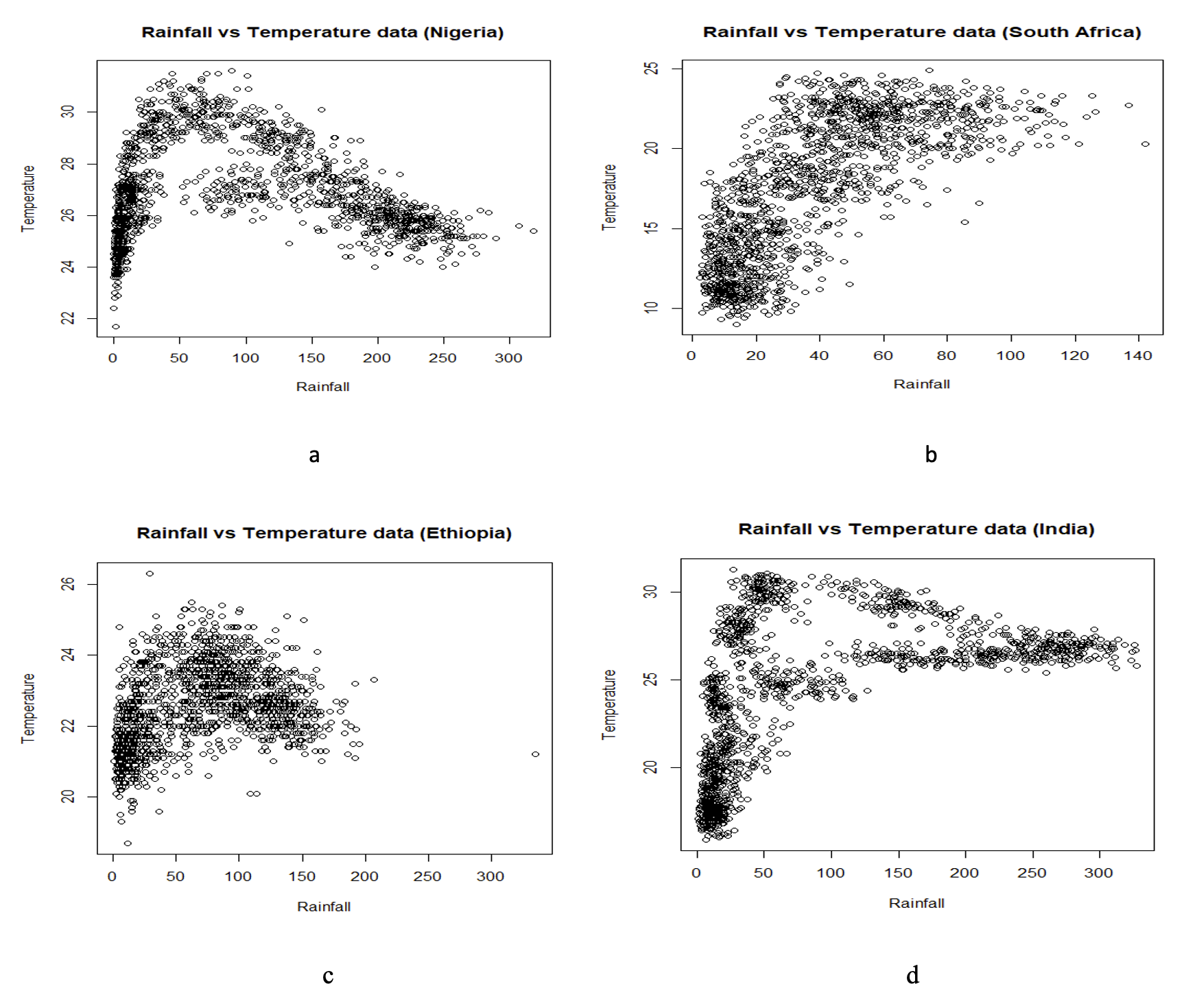
The bivariate relationship between the mean temperature and rainfall for the four selected countries is plotted in Figure 1. An eyeball observation indicates that each one has a distinct shape with Nigeria having the most pronounced hyperbola-like non-linear relationship. A further look suggests a similar shape between Nigeria and Ethiopia and then between South Africa and India. In the following sections, we will see if this similarity translates into similar attributes in the pairs.

Figure 1.Bivariate plot of temperature against rainfall in Nigeria (a), South Africa (b), Ethiopia (c ) and India (d).

Based on quantiles, the following three compound climatic zones are identified on each bivariate plot namely, dry-hot (DH), wet-warm (WW) and extreme dry-cold (EDC). For the DH, two cases are studied which are weak dry-hot (WDH) and the strong dry-hot (SDH). The former refers to the union of the rainfall and temperature observations where they exceed a threshold in either one or both margins while the latter implies the intersection of the observations where they simultaneously exceed both thresholds at the same time (here, the rainfall-temperature ratio will be computed). The WDH is taken as the independent case while the SDH, the dependent case. The chosen quantiles and their respective results are displayed on Table 1.

The historical distributions of rainfall and temperature in each of the selected separate modes are clearly reflected in the histograms in Figures 2, 3 and 4. With respect to the dry-hot zone, South Africa and India (Figure 2c and g) have similar rainfall distributions (which is closer to the normal distribution), likewise, Nigeria and Ethiopia are much the same (Figure 2a and e). However, in the hot condition, all countries display comparable distributional characteristics (Figure 2b, d, f and h). That is, they are all right-skewed but with slightly different tail structures in terms of how fast/slow they decay. There are no significant jumps at the tails.

Figure 2.The historical distribution of rainfall in dry condition (left) and temperature in hot condition (right) across the selected countries.

The extreme dry-cold histograms in Figure 3 distinctly showcase the similarities between Nigeria and Ethiopia and between South Africa and India in both the dry (for rainfall distributions) and cold (for temperature distributions) conditions. Figures 3b and f suggest that in the event of extreme dry-cold condition, temperature will play a more significant role in Nigeria and Ethiopia while rainfall will have more impact in South Africa and India. The left-skewed distribution for the former pair is indicative of a steady rise in cold temperatures.

Figure 3.The historical distribution of rainfall in extreme dry condition (left) and temperature in extreme cold condition (right) across the selected countries.

In the wet-warm division (Figure 4), the distribution of South Africa’s temperature (Figure 4d) is uniquely different from the other countries. It is like a mix of a left-skewed and a right-skewed distribution. That of Nigeria (Figure 4b) suggests a bi-modal structure as two significant peaks can be seen. The rainfall in India (Figure 4g) is indicative of a protracted tail which may signify an extended period of heavy rainfall (on average) in the wet season.

Figure 4.The historical distribution of rainfall in wet condition (left) and temperature in warm condition (right) across the selected countries.

4.1. Independent cases

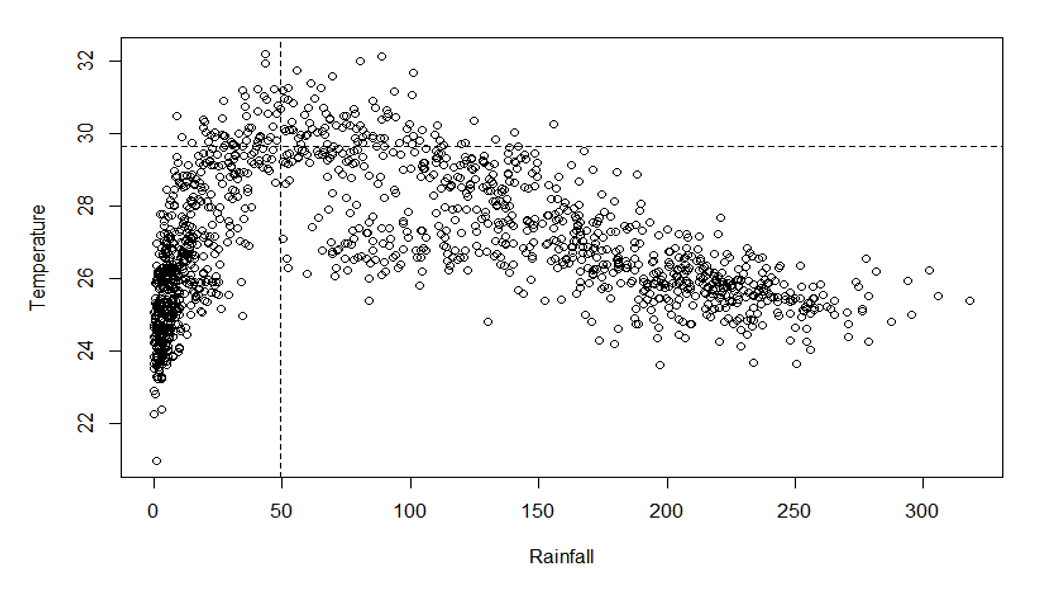
The corresponding observations in each zone are extracted and randomized. Within the independent context, the number of rainfall and temperature differ in most cases. For instance, the domain (D*) for weak dry-hot (Nigeria, Figure 5) is the region with the union (U) of rainfall (R) and temperature (T) variables as denoted by D*={(R, T): R<49.29430mm U T>29.66377 ⁰C}.

Figure 5.Scatter plot showing the dry-hot regions of rainfall and temperature in Nigeria.

This will cover observations in the first, second and third quadrants (clockwise) giving the numbers 584 and 140 for rainfall and temperature, respectively. The correlation between the variables is thus achieved by resampling the same number of the smaller observations (in this case, temperature) from the larger observations (that is, rainfall in this case) and taking the correlation. This is repeated a large number of times (n =1000) and the mean of n is taken, thereby giving every rainfall observation an equal chance to be selected. The results of the correlation for temperature and rainfall in the different compound climatic zones are presented in Table 2. These all represent the weak cases.

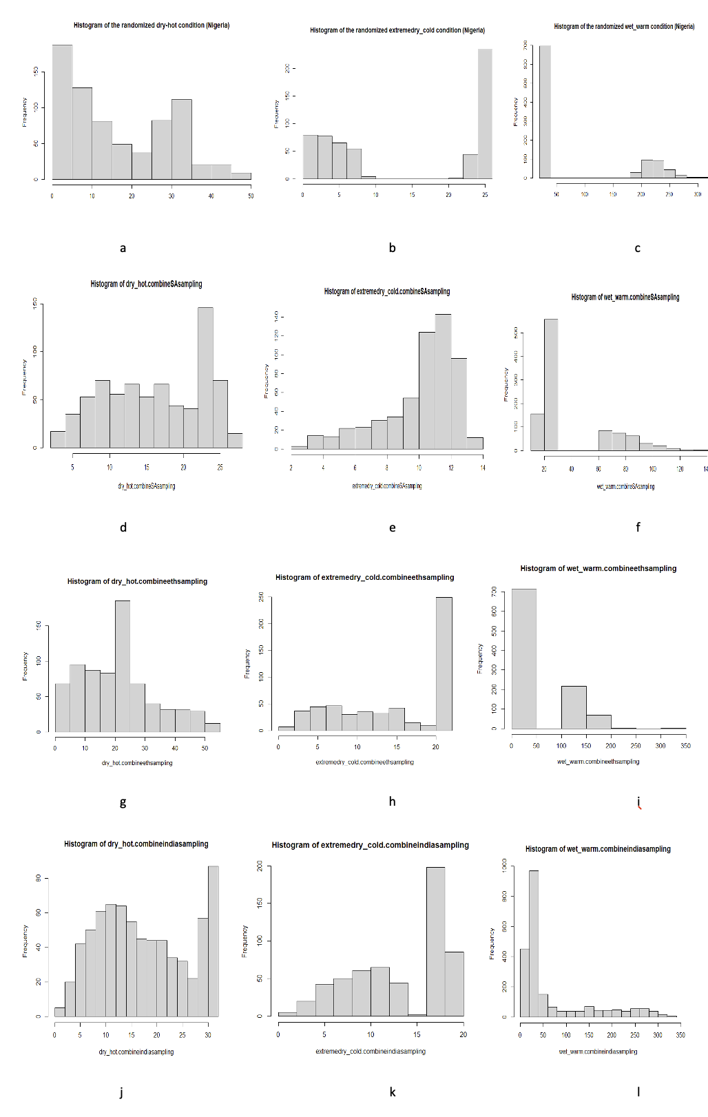
The simulated distributions of the combined randomized rainfall and temperature variables in each zone are provided using histograms in Figure 6. The corresponding plots of the climatic waves are given in Figures 7, 8 and 9. These are termed randomized variability plots. It is generally observed that the dense portions of the randomized variability plots which lie either at the bottom, top or mid-section correspond respectively to right-skewed, left-skewed or normal-like distributions.

Figure 6.Combined rainfall and temperature variables in the climatic zones of weak dry-hot (left), extreme dry-cold (middle) and wet-warm (left).

The first to fourth rows respectively correspond to the countries Nigeria, South Africa, Ethiopia and India.

The dry-hot and extreme dry-cold environment or season for all the countries (Figure 6a, d, g and j) generally depicts high jumps at their tail end indicating some level of significant severity of the condition. Additionally, they are mostly left-skewed (with the exception of Nigeria) while only the wet-warm zones are right-skewed. Some interesting distributions include that of India’s weak dry-hot zone (Figure 6j) where the core conforms to a Gaussian-like distribution but with a major spike at the tail. Also, its wet-warm structure (Figure 6l) exhibits a long-tailed distribution (roughly exponential) which is more or less uniform, hence less volatile but with a steady continuous drawn-out effect. Moreover, it is the only distribution that presents a fused climatic pattern under the wet-warm season.

South Africa’s denseness is at the top (Figure 7b), an indication of its left-skeweness (which although, is not so pronounced). The extreme dry-cold modes (Figure 8) are denser at the top and less at the bottom. This corresponds to the left-skewed structure in Figures 6b, e, h and k.

Figure 7.Climatic signals in weak dry-hot environment.

Figure 8.Climatic signals in weak extreme dry-hot environment.

The Nigerian extreme dry-cold pattern (Figure 8a) is quite different. It reveals quite a number of pocket spaces, straight-like lines and a denseness that spreads across (although, not too evenly). This same pattern (in reverse) is reflected in Figures 9a, b and c (with the more dense regions at the base).

Figure 9.Climatic signals in weak wet-warm environment.

When compared to figure 6, it can be observed that this pattern is reflective of histograms that showcase two separate disconnected sections.

4.2. Dependent case for dry-hot

The strong dry-hot as noted takes on observations of rainfall and temperature that lie simultaneously in the same zone. From Figure 5 (for Nigeria) this will refer to the domain (D**) in the second quadrant with the intersection of rainfall (R) and temperature (T) in D**={(R, T): R<49.29430mm, T>29.66377 ⁰C}.

In Table 3, the number of observations in each SDH division for each country is shown. Only Nigeria and Ethiopia have a significant number. It can also be observed that the correlation of the variables in this SDH zone is much higher than that of the weak dry-hot zone as indicated in Table 2. In fact, in the case of Nigeria, it is way much higher - a correlation of about 34% under the dependent assumption for dry-hot climatic division in contrast to the independent case assumption having correlation of <1%.

According to Cosmulescu and Gruia (2016), the ratio of rainfall to temperature should be (in general) equal or greater than 3.0mm/⁰C to enable a suitable condition for crops to grow. This is the ratio that will be (weakly) adopted for the SDH zone.

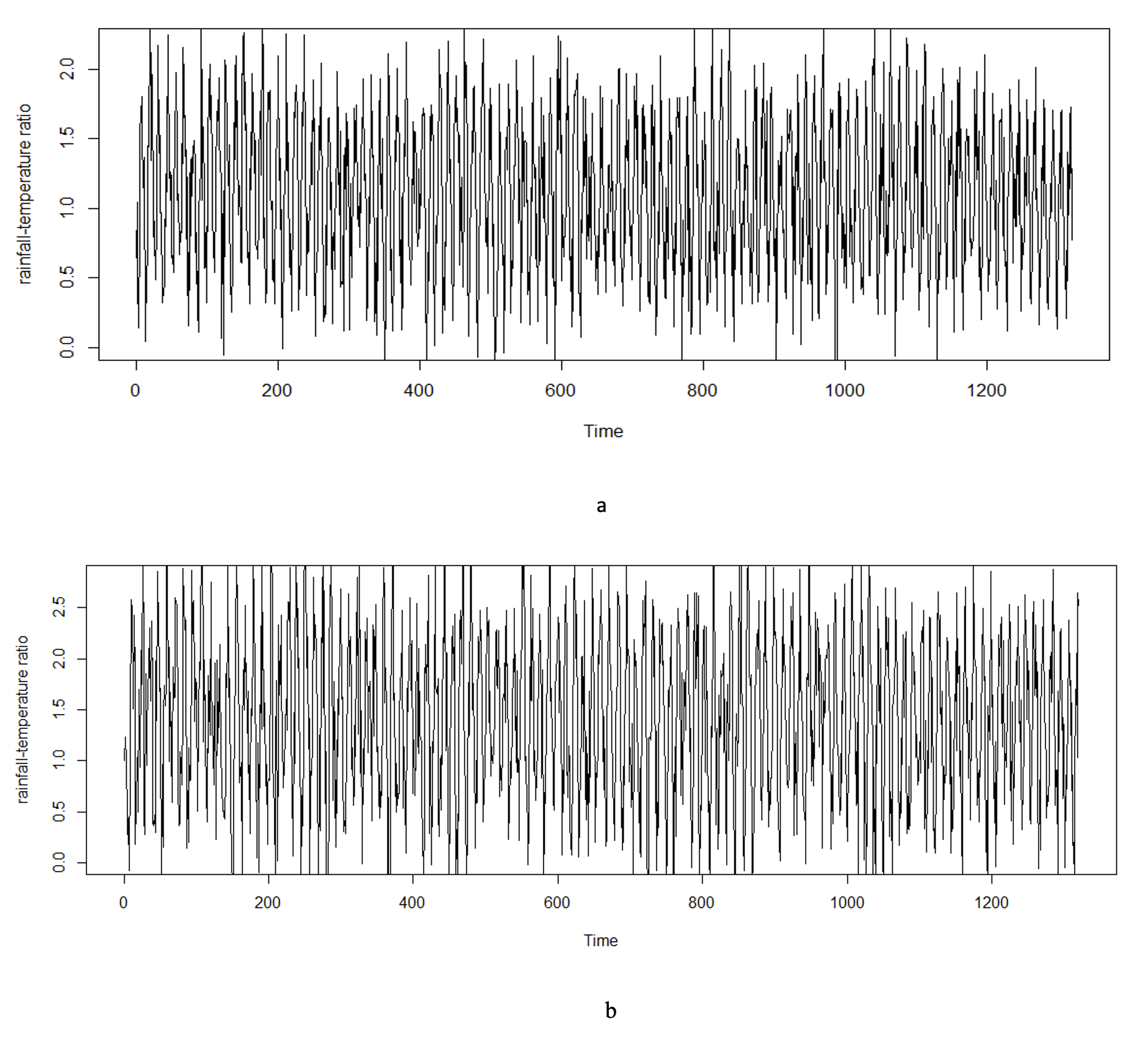
A slightly rising trend can be spotted between rainfall and temperature in the local regression plot (Figure 10b) for Nigeria, but the ratio of the variables showcases a slightly decreasing trend (Figure 10a). The reverse is the case for Ethiopia, the ratio of the variables displays an increasing trend but the relationship between rainfall and temperature is quite stable (Figure 10c and d). The sudden jumps in both cases (Figure 10b and d) are also reflected in the histograms (Figure 11) where Nigeria peaks at the tail end and that of Ethiopia is more at the mid-section. Overall, both distributions have a similar shape as confirmed by the simulated series plot (Figure 12).

Figure 10.Rainfall-temperature ratio (left) and temperature against rainfall (right) for Nigeria and Ethiopia.

Figure 11.Histogram representing the ratio of rainfall to temperature distributions in Nigeria (a) and Ethiopia (b).

Figure 12.Simulated climatic signals in strong dry-hot environment.

This series is achieved by sampling 1,000 observations with replacement. The mean (standard deviation) is further obtained giving 1.094509 (0.3334203) for Nigeria and 1.410073 (0.4977872) for Ethiopia.

4.3. Modeling the strong dry-hot climatic signals

The SDH zone has special implications for drought-related scenarios and water crises, hence it is further given a greater attention in this section. According to Stallinga and Khmelinskii (2014) and Stallinga (2018), the climate can be treated as signals and thus modeled. Following in same vein, the variability of the SDH state will be treated as climatic signals and thus modeled using a combination of the simple harmonic motion and white noise techniques. The white noise parameters are the mean and variance of SDH variables in each country case (Nigeria and Ethiopia), the period (T) is taken as 12 indicating a monthly cycle. The time in months (t) runs from t=1 to t=1320 since there are 1320 months. The initial amplitude values are obtained from eyeball inspection of Figure 12 giving 0.6 for Nigeria and 0.9 for Ethiopia. Figure 13 shows the modeled SDH climatic signals.

Figure 13.Generating signals of strong-dry hot zone using trigonometric functions to obtain a sinusoidal input signal for Nigeria (a) and Ethiopia (b).

The more accurate amplitude is obtained by breaking the complex wave signal into two simple harmonic sinusoidal waves as expressed in equation (2) and then, linear regression is applied to obtain the omega values. The results are shown in Table 4. Since a negative amplitude simply implies that the wave starts from the opposite turn and does not change the characteristics of the signal, the absolute value of the amplitudes is adopted.

The sinusoidal function representing the Nigerian SDH zone can thus be written,

$$X_{t} = 0.61 \cos(\frac{2\Pi}{12}\ t - 1.26\Pi) + w_{t}(\mu = 1.0945,\sigma = 0.333)\tag{3}$$

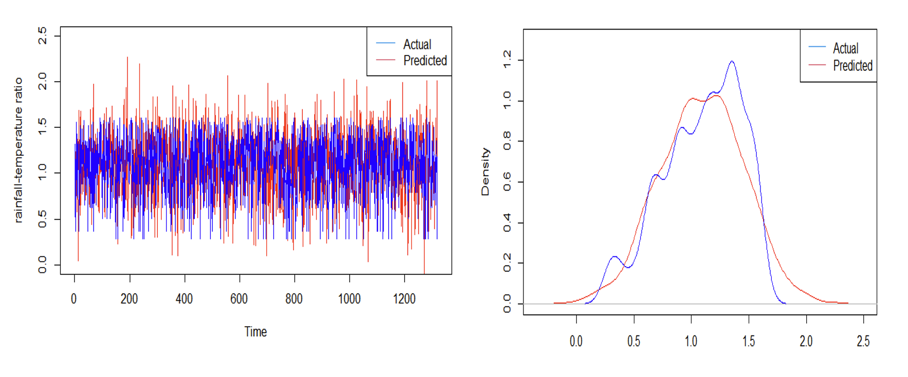
4.3.1. Comparing the empirical and fitted models (for the Nigerian case)

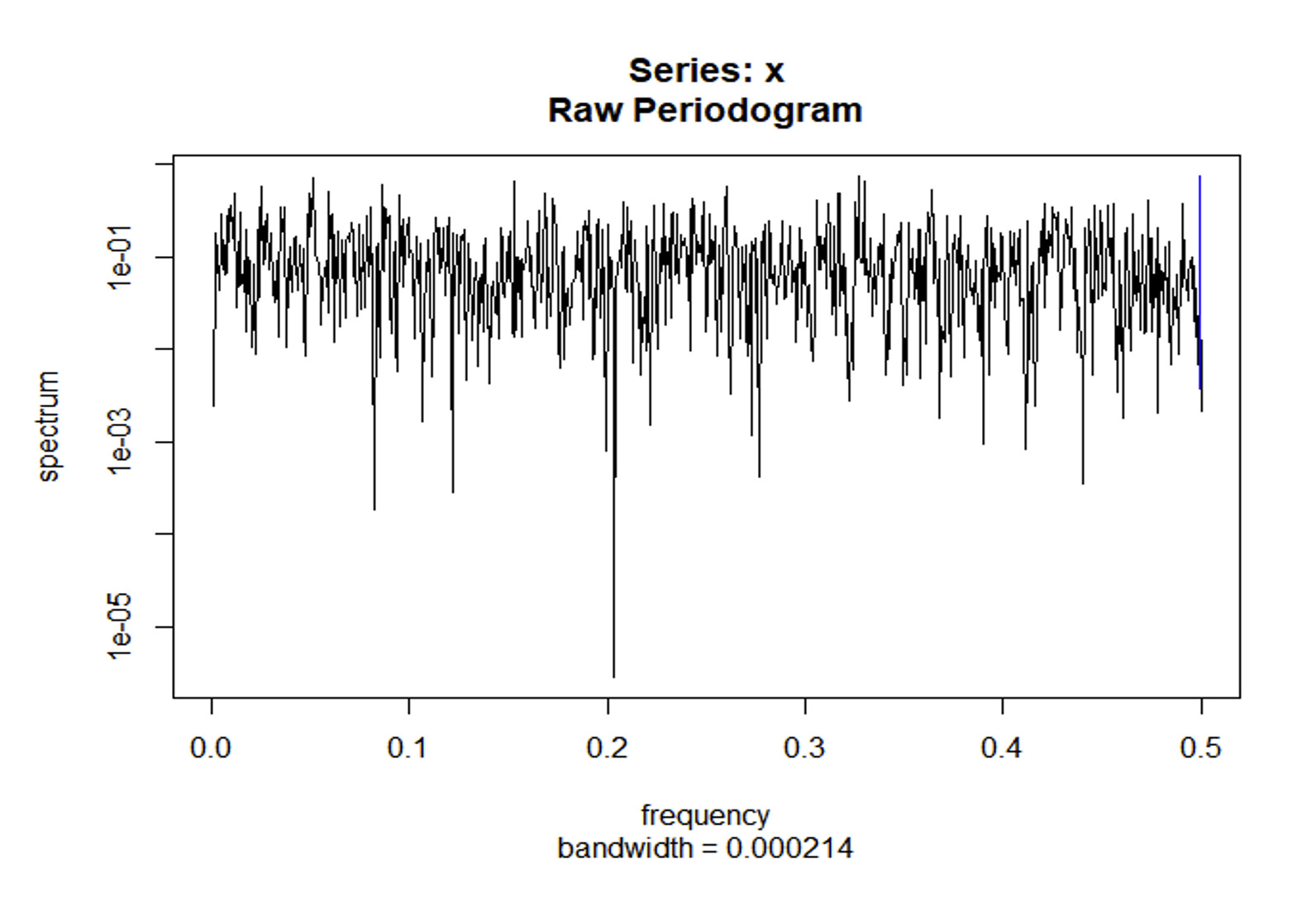
The goodness-of-fit graphs (Figure 14) based on equation (3) indicates that the fit still requires some improvement therefore the spectral density (Figure 15) for the specific SDH region/quadrant is further analyzed to obtain the exact maximum frequency (0.32667) which when inverted provides us with the quadrant-specific period given as T=3.061224. This is the period that will now be used instead of the generalized period (T=12).

Figure 14.Time series (left) and density (right) plots of predicted model (using equation 3) on empirical (actual) model.

Figure 15.Spectral density estimate using a periodogram that showcases the relative strengths of the various frequencies of the sampled SDH region.

Further adjusting the amplitude and scaling the Gaussian noise as noted in equation (4), a more improved model is realized (Figure 16).

$$X_{t} = 0.1 \cos(\frac{2\Pi}{3.06} t - 1.26\Pi) + 1.1w_{t}(\mu = 1.0945,\sigma = 0.333)\tag{4}$$

Figure 16.Density plot of predicted model in red (using equation 4) on empirical model in blue.

However, it was observed that the right tail was consistently being overestimated by a significant margin. As such, other noises were tested.

1. The mean and variance adjusted Gaussian noise.

$$X_{t} = 0.1 \cos(\frac{2\Pi}{3.06} t - 1.26\Pi) + 1.1 w_{t}(\mu = 0.0968,\sigma = 0.307)\tag{5}$$

This adjustment allows the full model’s mean and standard deviation to be similar to the empirical mean and standard deviation unlike the model in equation (4) (whose noise will now be termed non-adjusted Gaussian noise) where the similarity only occurs within the noise portion.

2. The skew-normal (SN) noise

A number of runs were made slightly adjusting the parameters each time to obtain a much better fit. The parameters in equation (6) provide the fit (in green) in Figure 17.

$$\small{ \begin{align} X_{t} &= 0.1 \cos(\frac{2\Pi}{3.06} t - 1.26\Pi) \\ &\quad + 1.3 {sn}_{t}(\mu = 1.0945,\text{scale} = 0.30, \text{alpha} = - 2.0, \text{tau} = 0) \end{align} \tag{6} }$$

Alpha is the slant parameter; tau is the hidden mean parameter for the extended SN (a zero indicates SN). Several runs of the models give slightly different results. One such realization is indicated in Figure 17 where the tested model densities and distribution functions are compared to the empirical model.

Figure 17.Density (left) and distribution (right) plots comparing the predicted models with the empirical (actual) model.

It can be observed that none of the single models adequately fitted the whole data. While they are a good fit in some sections, they tend to overfit/underfit in other sections. For instance, the sinusoidal model with SN noise fits better at the right tail portion but overestimates the peak value. This was further confirmed by the Kolmogorov Smirnov (KS) goodness-of-fit two-sample test (Table 5). The p-value in each case is less than the chosen significant level (0.05).

Nevertheless, by comparing the quantiles, we see quite close approximations of the specific models at different sections in comparison with the empirical model (Table 6). This possibly suggests that a mixture model which combines any two or even the three indicated models could provide a much more improved fit.

4.4. Setting a baseline compound climatic zone

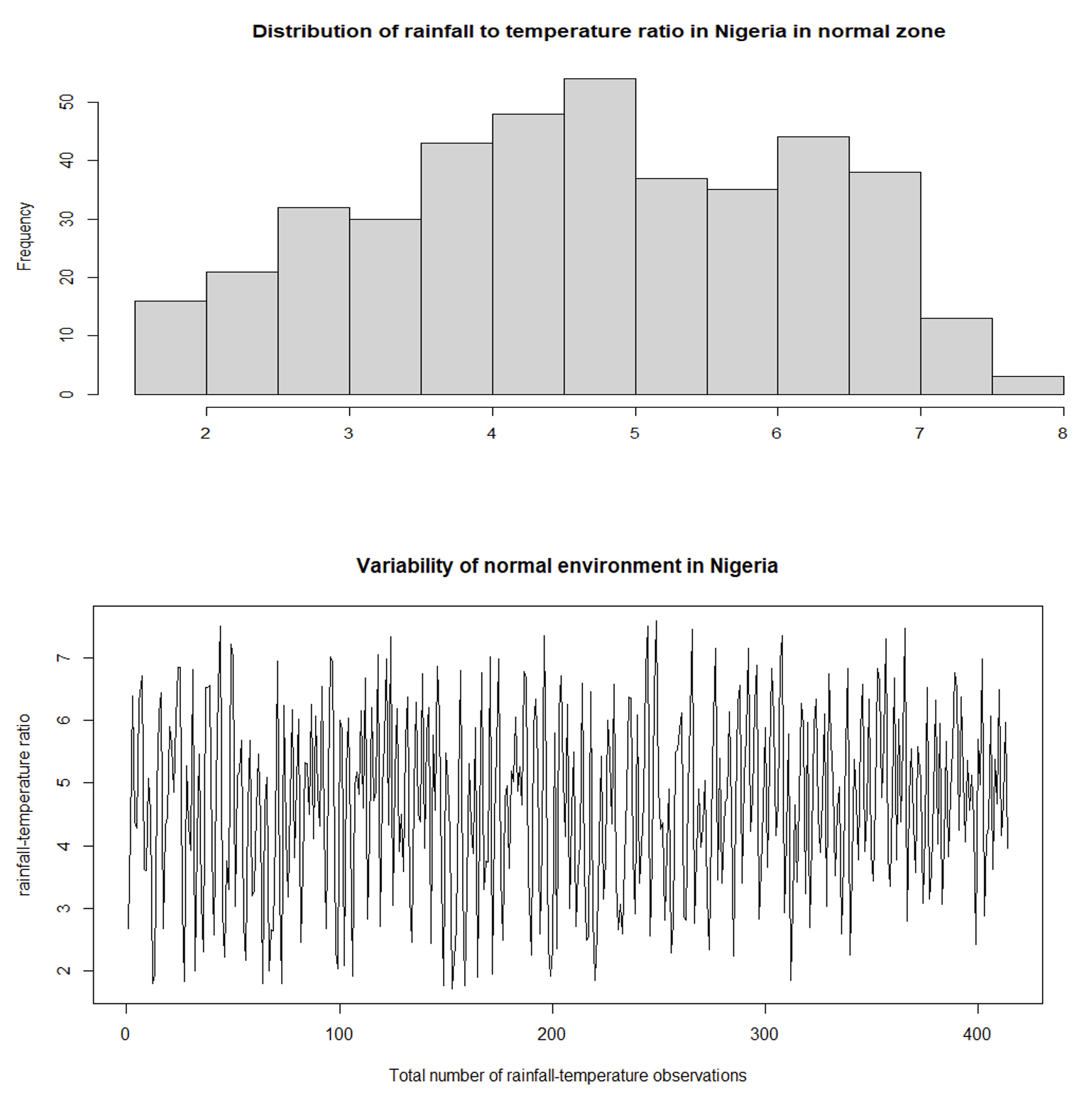
There is a need to have a reference compound climatic zone which can be used as the baseline or yardstick with which other zones can be compared to. The normal zone where the rainfall and temperature are in the right proportion for optimal crop growth (in a general sense) is adopted. Only the Nigerian case is considered. The choice of the normal range for rainfall and temperature is based on Figure 18 which suggests that the dry season falls within the months January, February, March, November and December which are mostly below 50mm. Additionally, Ajetomobi (2016) showed that maximum temperatures between 30 ⁰C and 35 ⁰C posed a high damage to crops like cassava, maize and cotton. Thus, the normal climatic division will be assumed to fall between 49-200mm for rainfall and between 26-29.66 ⁰C for temperature.

Figure 18.Average rainfall amount in Nigeria aggregated by months (1901-2020).

In this zone, a clear negative relationship between rainfall and temperature can be clearly observed (Figure 19) and the ratio of rainfall to temperature depicts a distribution that is similar to a normal distribution (Figure 20). In the normal zone, the ratio of rainfall to temperature is higher than in the dry-hot division. More precisely, approximately 86% of the rainfall-temperature ratio values are greater than 2.8 mm/⁰C in comparison to the strong dry-hot zone where same proportion of observations are not greater than 1.6mm/⁰C.

Figure 19.Scatterplot (left) and local regression plot (right) of rainfall and temperature in the normal climatic zone.

Figure 20.Normal climatic distribution (above) with the corresponding wave plot (below).

Comparing the simulated wave signal of the compound climatic normal zone to that of the SDH zone (Figure 21), a difference can be noted with respect to the dense locations in the plot - mid section for the normal case and top section for SDH case. Additionally, their long-run means differ significantly, 4.6579 mm/⁰C for normal and 1.0945mm/⁰C for SDH.

Figure 21.Simulated climatic signals in normal environment (above) and the strong dry-hot zone (below) for Nigeria.

6.0. Conclusion

The dry-hot, extreme dry-cold and wet-warm compound climatic conditions in four countries in Africa and Asia were compared and contrasted. It was generally observed that South Africa and India share more similarities in their rainfall-temperature distributions. In order to model the climatic variability in the strong dry hot region (for Nigeria), the sinusoidal model in combination with several noises were tested. Some of the models differ at the center of the distribution while some differed at the tail region. By observing and comparing the quantile estimates, this paper shows that there is an indication that a mixture of any of the tested models could provide a much better wholesome fit. This is a highlighted path for future studies.

Acknowledgement

The author thanks the reviewers at CAS for their insightful comments.

Author’s Biography

Dr. Queensley C. Chukwudum is a first-class graduate of mathematics/computer science from Federal University of Technology, Minna and the best graduating MSc. mathematics student from the University of Jos (2008/2009 session) in Nigeria. She obtained her PhD in financial mathematics from the Pan African University Institute for Basic Sciences, Technology and Innovation (PAUSTI) in Kenya under the African Union scholarship and has a postgraduate diploma in actuarial science from the University of Leicester, UK. Professionally, she has over 10 years of teaching experience. Currently, she works at the Department of Insurance and Risk Management, University of Uyo, Nigeria, where she teaches business mathematics/statistics, computer application and risk management at the undergraduate level while at the post graduate level she teaches reinsurance and, insurance laws & regulations.

Her research activities include extreme value analysis in African financial markets and climate change issues, claims and portfolio analyses as well as data analytics. She has published a couple of papers in top-tier journals and has participated in high-ranking conferences. She has received a number of awards such as the 2019 Pan African winner of the African Union’s ‘My thesis in 180 seconds’ competition. Her research contribution in climate change has earned her the Allianz Climate Risk Research Award and the African Institute for Mathematical Sciences Women in STEM recognitions in 2019. She is also a recipient of the UK-Africa Postgraduate Study Institute in Mathematical Sciences scholarship and was recently awarded the Massachusetts Institute of Technology Chief Data Officer and Information Quality (MIT CDOIQ) of her Institute (University of Uyo) by the MIT Country CDOIQ of Nigeria.

Queensley is a fellow of the Institute of Information Management, Africa and the Institute of Management Consultants, Nigeria. She is the current Chair of the Southern Africa Mathematical Sciences Association (SAMSA)-MASAMU Pan-African research group on Insurance and Climate.