1. INTRODUCTION

Smoothing “bumpy” or “volatile” data is not required in many actuarial analyses. However, it is often needed when rating factors vary by policy limits, amount of insurance, or other characteristics that fall into “buckets” along a line, or when a random sample is used to construct a severity distribution. Typically, the average frequency, severity, pure premium, percentage of sampled values, etc. of all the risks that fall into each bucket is the value assigned to the bucket, and for smoothing purposes the index assigned to each bucket is the midpoint of the range of the amount of insurance, etc. that the bucket covers.

Smoothing is especially relevant when the data in some or all of the buckets do not have adequate credibility. This paper begins with a credibility-based approach to smoothing that recognizes the credibility of individual buckets but still recognizes the tendency of a curve to move in a continuous way and at a continuous rate. Then, it expands the method to provide a broader tool kit for more challenging smoothing situations.

2. THE MODEL

This approach begins with a model that reflects certain assumptions. The situation, in more precise terms, is:

• The data in each of the buckets has what might be termed process variance around the true, but unknown, values along an underlying curve. The data creates a statistical approximation to that curve which is more accurate at the points/buckets^[1] where there is more data (less process variance) and less accurate elsewhere.

• The underlying curve is assumed to be fairly smooth, so the point-to-point changes on the underlying curve would be encouraged, but not forced, to change by the same slope as one moves along the curve.

• On the other hand, most curves do not fall perfectly along a line, so the point-to-point changes along the curve should have random aspects but still retain a continuous looking shape.

• Further, few actual curves seen in practice are generated from straight lines or linear relationships, so that trend must change as one moves from point to point along the curve.

• However, one would logically assume that the process errors, the general trend, and the point-to-point trends between adjacent points are all random.

Then, the next step is to develop a model that may be used to estimate the curve by smoothing the data.

2. THE SIMPLER MODEL-CONSTANT UNDERLYING TREND

In this model, the process error variances vary from point to point but are either known or estimated with reasonable accuracy. Under best estimate credibility (see Boor 1992) that process error would be part of a multiplicative inverse of credibility. So, points with high process error should receive less weight in deriving the smoothed curve. Then, to illustrate the situation, there would be observed data points \(\mathbf{S}_{\mathbf{1}}\mathbf{,\ }\mathbf{S}_{\mathbf{2}}\mathbf{,\ \ldots,\ }\mathbf{S}_{\mathbf{n}}\mathbf{\ }\)that differ from the unknown true values \(\mathbf{p}_{\mathbf{1}}\mathbf{,\ }\mathbf{p}_{\mathbf{2}}\mathbf{,\ \ldots,\ }\mathbf{p}_{\mathbf{n}}\mathbf{\ }\)by process errors with variances of \(\mathbf{\sigma}_{\mathbf{1}}^{\mathbf{2}}\mathbf{,\ }\mathbf{\sigma}_{\mathbf{2}}^{\mathbf{2}}\mathbf{,\ \ldots\ ,}\mathbf{\sigma}_{\mathbf{n}}^{\mathbf{2}}\mathbf{\ }\)respectively.

If one defines each “change”\(\mathbf{\ D}_{\mathbf{i + 1}}\mathbf{\ }\)as the change from point-to-point \(\mathbf{\ D}_{\mathbf{i + 1}}\mathbf{=}\mathbf{\ p}_{\mathbf{i + 1}}\mathbf{-}\mathbf{p}_{\mathbf{i}}\), one might view them as driven by trend. That is especially in this case where the data is evaluated at the points 1, 2, …, n, or other situations where the indices (\(\mathbf{i'}\)s) are equally spaced. The expected trend is assumed to be constant, at some slope \(\mathbf{G}\). However, since one would not expect the underlying values to lie perfectly on a line, one must allow the actual (and also unknown) changes to vary from period to period around \(\mathbf{G,}\) with some variance \(\mathbf{\tau}^{\mathbf{2}}\mathbf{.}\)

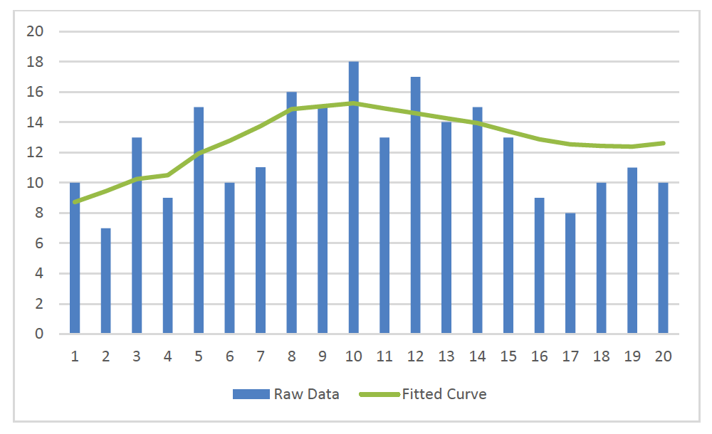
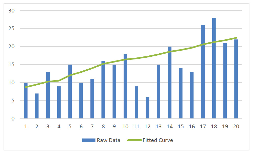
Table 1 shows an example of the consequent smoothing process. The assumed constant overall trend (not yet the ghost trend) of, in this case, 0.75, is specified in column (7). The process variances are specified, along with the observed values, \(\mathbf{G}\) =0.75, and \(\mathbf{\tau}^{\mathbf{2}}\mathbf{=}\) 0.80. The actual data values input to the process and estimates of their variances around the “true” underlying expected values are included in columns (2) and (3). The fitted curve, the '\(\mathbf{p}_{\mathbf{i}}\)‘s’ that the process finds are in column (4). The normalized fit error (the squared differences between the raw data and the \(\mathbf{p}_{\mathbf{i}}\)'s, divided by the variance associated with the raw data point) is computed in column (5). The estimate of the “local” (using \(\mathbf{p}\) between the \(\mathbf{(i - 1)}^{\mathbf{th}}\mathbf{\ }\)and \(\mathbf{i}^{\mathbf{th}}\mathbf{\ }\)steps) trend is computed in column (6). The constant overall governing trend (in this case, 0.75) is posted in column (7). Lastly, how far the “local trend” has "drifted away from that constant trend is computed by taking the squared difference between the local trend and the selected overall trend value, the dividing the results by a common preselected, \(\mathbf{\tau}^{\mathbf{2}}\mathbf{=}\).8. That result is shown in column (8).

Then the goal is to find the \(\mathbf{p}_{\mathbf{i}}\)'s that simultaneously fit the data well and yet provide a smooth curve. However, the values of “does not fit the data well” and “is not smooth,” are easier to compute numerically than the original targets. Specifically, the sum of all the entries in column (5), the normalized fit error, represents “does not fit the data well .” The sum of the entries of the drift in the local trend in column (8) represents “is not smooth ,” albeit indirectly. Then one would seek to reduce (minimize, speaking in numerical terms) those values.

Essentially, using a computer minimization routine, the process finds the \(\mathbf{p}_{\mathbf{i}}\mathbf{\ }\)points that minimize the standard squared differences(squared difference divided by variance) between the points and the observed data, the \(\mathbf{S}_{\mathbf{i}}\)'s. It simultaneously minimizes the standard squared differences between the \(\mathbf{\ p}_{\mathbf{i + 1}}\mathbf{-}\mathbf{p}_{\mathbf{i}}\)'s and \(\mathbf{G}\) as well. First, a cell or variable adding together the subtotals of columns (5) and (7) is now included in the chart and highlighted in yellow. Then the value in that target cell in yellow was minimized by finding the\(\mathbf{\ p}_{\mathbf{i}}\)'s that create the lowest possible value of the target. For reference, the solution routine in standard spreadsheet software was used to compute the \(\mathbf{\ p}_{\mathbf{i}}\)'s in all of the tables in this article.

In this case, the fitted curve looks like it could reasonably be a smoothed version of the data. However, in this special case, the data does show a steady uptick, mirroring the assumption of constant governing trend. Hence, something similar to a straight line can be an effective smoothing of this particular data.

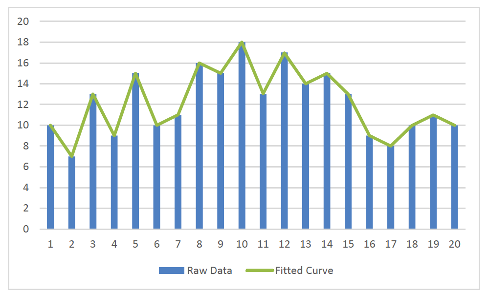
On the other hand, when the raw data has a ‘hump,’ or other curvature, the results of this smoothing method do not fit the data as well. In Figure 2 all the parameters are exactly the same as they were in Table 1 and Figure 1, (except for minimizing the target “C” by selecting new\(\mathbf{\ p}_{\mathbf{i}}\)'s) but the raw data values are more U-shaped.

Figure 1.Fitted vs. Raw Data

Figure 2.Fitted vs. Raw Data with ‘Hump’

Of course, some of the fit problems may be mitigated by changing the values of the drift parameter \(\mathbf{\tau}^{\mathbf{2}}\) and the expected trend \(\mathbf{G.}\) One may vary both those, as well as the various \(\mathbf{p}_{\mathbf{i}}\)'s to produce a better match to the data. In fact, varying those values produces the following graph (reusing the Figure 2 raw data).

However, one may readily see, that this eliminates all smoothing. Considering the alternatives, the use of constant expected trend in the simple model limits its ability to appropriately smooth data with “humps.”

3. INCLUDING THE GHOST TREND

Since the constant underlying trend \(\mathbf{G}\) limits the ability of the smoothing process in Section 2 to mimic curves, it would be logical to enhance \(\mathbf{G}\) by allowing it to change as one moves among the data points. Therefore, one would no longer specify a constant expected trend (as Table 1 did), but rather find the expected local trends that best match the data. Of course, there should be some control on the point-to-point changes, or something like Figure 3 will reoccur. The result is that one will have a set of “nearly invisible” \(\mathbf{G}_{\mathbf{i}}\)'s, governed by a requirement that the difference between each \(\mathbf{G}_{\mathbf{i}}\) and \(\mathbf{G}_{\mathbf{i + 1}}\) follow a probability distribution (in this article they are specified to vary with a mean of zero and a constant variance of some \(\mathbf{\delta}^{\mathbf{2}}\mathbf{)}\). The \(\mathbf{\ D}_{\mathbf{i}}\)'s would continue to vary around \(\mathbf{G}\), except that now each \(\mathbf{\ D}_{\mathbf{i}}\mathbf{\ }\)will vary around each individual \(\mathbf{G}_{\mathbf{i}}\mathbf{\ }\)with mean zero and a variance of some prespecified \(\mathbf{\tau}^{\mathbf{2}}\).

Figure 3.Choosing All Parameters to Minimize Variance

The unobserved, indirectly estimated, and “nearly invisible” \(\mathbf{G}_{\mathbf{i}}\)'s affect the \(\mathbf{\ D}_{\mathbf{i}}\)'s the \(\mathbf{\ D}_{\mathbf{i}}\)'s help to determine the\(\mathbf{\ }\mathbf{p}_{\mathbf{i}}^{\mathbf{'}}\mathbf{s}\mathbf{,\ }\)and those smooth the \(\mathbf{S}_{\mathbf{i}}\)'s, which in turn are the only hard data in the process. So, in a sense, the \(\mathbf{G}_{\mathbf{i}}\)'s are shadows of shadows of the data. It is then logical to describe them as “ghost trend.”

In this case, the total standard squared error to be minimized still includes that of the differences between the \(\mathbf{p}_{\mathbf{i}}\)'s and the \(\mathbf{S}_{\mathbf{i}}\)'s and that between the \(\mathbf{\ D}_{\mathbf{i}}\)'s and now the \(\mathbf{G}_{\mathbf{i}}\)'s. However, it also includes the squared differences (divided by\(\mathbf{\ }\mathbf{\delta}^{\mathbf{2}}\mathbf{)}\) arising between each \(\mathbf{G}_{\mathbf{i}}\mathbf{\ }\)and the \(\mathbf{G}_{\mathbf{i - 1}}\) that preceded it. Table 2 illustrates this process.

To implement the ghost trend process, the chart in Table 2 adds two columns to the chart from Table 1. The constant trend in the previous example is replaced with a column (7) of ghost trend. To keep the ghost trend smooth, a “penalty” column, containing the squares of the differences between successive values of the ghost trend is included as column (8). To control the balance between that column, the fit error penalty column (5), and column (9) penalizing the drift of the actual trend (\(\mathbf{D}_{\mathbf{i}}\)'s) from the “expected” ghost trend (\(\mathbf{G}_{\mathbf{i}}\)'s), each term in column (8) is divided by the \(\mathbf{\delta}^{\mathbf{2}}\) discussed above.

Further, in this case, the sum of the fit error, the drift penalty, and the ghost trend smoothing penalty must be computed in the target cell/variable to be minimized. So, the total variance in C. below (in yellow) sums all three. The spreadsheet minimization routine was directed to minimize that value by choosing the values of the \(\mathbf{\ p}_{\mathbf{i}}\)'s and \(\mathbf{G}_{\mathbf{i}}\)'s in columns (4) and (7). The results are shown in Table 2. Of course, the key values are the smoothed values, the \(\mathbf{\ p}_{\mathbf{i}}\)'s, in column (4).

As one may see in Figure 4, this provides a better fit (conforms better) to the last half of the data from Figure 3.

Figure 4.Ghost Trend vs. Fixed Expected Trend

Figure 5.Ghost Trend vs. Fixed Expected Trend on Steep Hump Using \(\mathbf{\ \delta}^{\mathbf{2}}\mathbf{= .0625}\)

Now, in this case, the hump is fairly modest. However, when a more pronounced hump (such as a normal distribution with a low variance) is involved, the difference may be more significant. Figure 6 looks at data with a steeper hump but continues using the existing \(\mathbf{\delta}^{\mathbf{2}}\) of .0625.

Figure 6.Ghost Trend vs. Fixed Expected Trend on Steep Hump Using \(\mathbf{\ \delta}^{\mathbf{2}}\mathbf{= 5}\)

In this case, the fit is improved, but still not that desirable. However, this approach also allows one to vary the “long-term flexibility” \(\mathbf{\delta}^{\mathbf{2}}\). When the \(\mathbf{\delta}^{\mathbf{2}}\mathbf{\ }\)parameter is increased to five in Figure 6, the fit is demonstrably superior to that of the simpler model.

Increasing\(\mathbf{\ \delta}^{\mathbf{2}}\) results in smoothing with a fairly good fit. This illustrates a key point. Both approaches require selecting two parameters. For the fixed expected trend approach, the trend and the short-term flexibility (or inverse of smoothness) parameter \(\mathbf{\tau}^{\mathbf{2}}\) must be selected. For the ghost trend, \(\mathbf{\tau}^{\mathbf{2}}\mathbf{\ }\)must still be chosen, but one also chooses the long-term flexibility parameter \(\mathbf{\delta}^{\mathbf{2}}\). Therefore, actual implementation may involve judgments of how much smoothness is desired and how much replication of the data, or “fit,” is required.

It would be desirable if some proper optimum set of parameters for smoothing could be identified, but, considering Figure 3, that appears to be impossible. Nevertheless, given proper judgment-based selections of the flexibility parameters, this appears to be a very good, structured, tool for smoothing data.

4. AN EXAMPLE: USING AN ENHANCED GHOST TREND ANALYSIS ON VERY CHALLENGING DATA

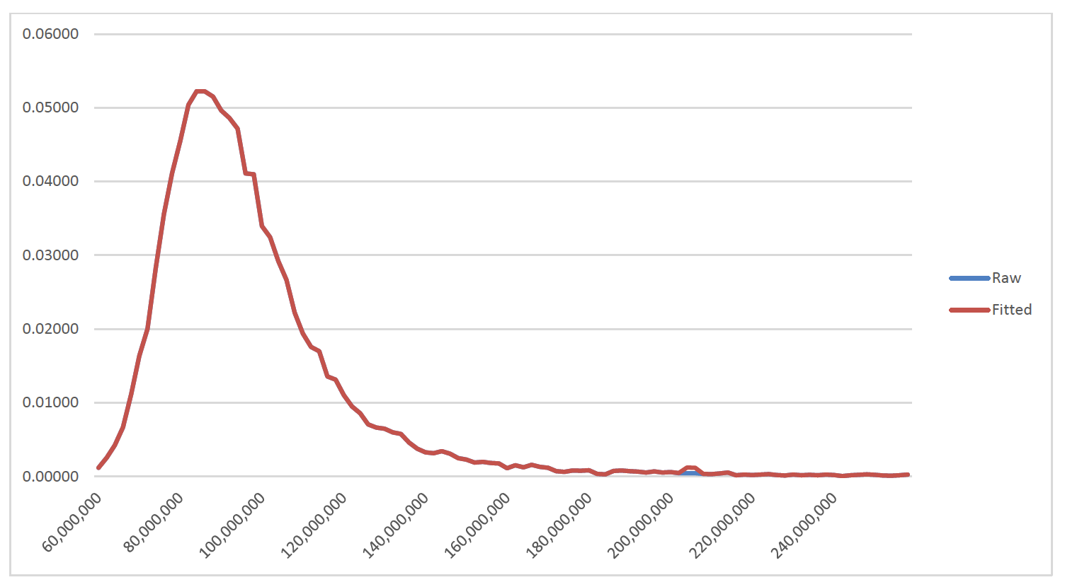
Sometimes fitting a curve can be difficult even when the ghost trend process is used. For example, in process of preparing a separate article related to assessing transfer of risk, Boor 2021, it was necessary to use an aggregate loss distribution with the number of claims generated by a Poisson random variable with a mean of five hundred and the severity distribution of each claim following a Pareto distribution with an alpha value of 1.5 and truncation point of 100,000. The simulation^[2] was not overly hard to generate. However, the results of the simulation, graphed in Figure 7, and supported by the data in Table 3, are fairly “bumpy ,” even after combining thirty thousand trials into one hundred bands. Due to the large number of bands, only the first and last ten rows of the table are shown

Figure 7.Raw Results of Aggregate Loss Simulation.

For reference, the labels correspond to the top ends of the buckets, which each have a width of $2 million. However, as one may see a shift of $1 million to the left would not meaningfully change the appearance of the curve.

(Also, less than 1% of the curve lies in the tail beyond this range. However, due to the skewness of the distribution, graphing that would place most of the attention where the fewest losses are.)

The next step is of course to use the ghost trend approach. The approach is identical to Table 3, but with more data and different values for the constants. Note that as the calculations unfold the rationale behind the specific constants used will become clear. The resulting graph (including the raw data it began with) is in Figure 8.

Figure 8.Comparison of Results of Initial Ghost Trend -Generated Curve to Raw Data.

As one may see, in this case, and with the given assumptions the ghost trend approach alone does not match this numerous and volatile raw data very well. The associated calculations are shown, again for the first and last ten rows, in Table 4.

Table 4 partially explains the poor fit in this case. Although the trend values are modified by values of \(\mathbf{\tau}^{\mathbf{2}}\) and \(\mathbf{\delta}^{\mathbf{2}}\), which may be titrated up and down for the desired degrees of “stiffness,” the impact of the fit error column (5) is greatly affected by the variances in column (3). Further, the sum of column (5) is much larger than that of column (8), but the effect of column (8) is increased by an “adjustment factor” (discussed below) of 2000, the trend controls in column (8) have roughly the same impact as the fit (or accuracy) controls. So, this may be thought of as a fifty/fifty balance between smoothness and fit accuracy. Note also for reference that the variance-based divisors\(\mathbf{\ }\mathbf{\tau}^{\mathbf{2}}\) and \(\mathbf{\delta}^{\mathbf{2}}\) are now applied at the bottom of each column rather than used in the calculation of the individual column entries.

As used above, some additional adjustment factors are also used. Certainly, one is needed for the fit error column. As it turns out, though, two additional columns are both helpful in controlling the accuracy and smoothness of the fitted curve. First, a review of column (5) will show that the fit errors that enforce accuracy are much lower in the upper end of the range. Therefore, since small changes in the smoothed values would not generate many changes in the total error value at the bottom of the chart, one might argue that there is less emphasis on accuracy in the upper end of the range. However, readers might desire a smooth curve the works in different contexts with different requirements. So, now there is an additional column, along with its own adjustment factor. In its calculation, the difference between each raw value and \(\mathbf{p}\) value pair is then divided by the raw value before the result is squared and divided by the variance. That will give more weight to the smaller values, for a more consistent fit.

Another adjustment is included in this version. Noticing the sort of “granular bumpiness” (a high degree of small, high slope, oscillations near the tail), a direct control against abrupt changes in the slope is now included in the new column (8). It is simply the squared difference between each slope \(\mathbf{G}_{\mathbf{i}}\) and the previous slope \(\mathbf{G}_{\mathbf{i - 1}}\). This penalizes abrupt changes in the trend/slope. The adjustment factor applied to the total of those values titrates its influence on the fitted curve.

Those adjustments result in the curve in Figure 9. Note that the general shape is somewhat close to acceptable, but there is still so much bumpiness that, within the scale of the graph, it cannot be distinguished from the raw data.

Figure 9.Comparison of Results of Ghost Trend with Three Adjustments to Raw Data.

That curve is generated by the process in Table 5. Again, in this case, all the normalizing divisions, by \(\mathbf{\tau}^{\mathbf{2}}\mathbf{,}\mathbf{\ }\mathbf{\delta}^{\mathbf{2}}\mathbf{,}\) etc. take place at the bottom of the Table.

To finish the curve, a different smoothing process, centered five-point averaging, was used. That produced the quite acceptable curve in Figure 10.

Figure 10.Comparison of Results of Five Point Averaged Enhanced Ghost Trend Curve with Raw Data.

For reference, a curve comparing the fit, with the scale above, of straight five-point averaging to this process is provided in Figure 11.

Figure 11.Comparison of Results of Five Point Averaged Enhanced Ghost Trend Curve with Raw Data.

As one may, due to the relatively small changes from point to point and the large volume of points, straight five-point averaging is almost or as good as the ghost trend+ process. However, the example is good as an illustration of the process, if not for optimizing the result.

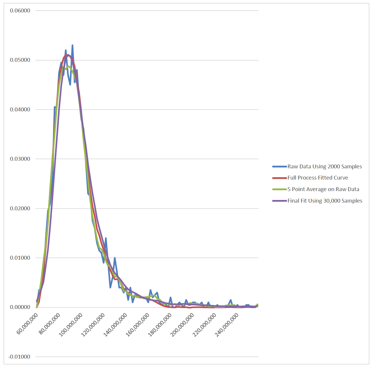
For an example where the ghost trend+ is clearly superior, one need only look at the same situation, only with 2000 points in the sample rather than 30,000.

Figure 12.Comparison of Results of Fully Enhanced 2000 Samples Ghost Trend Curve with Five Point Averaged Raw Data, Raw Data, and 30,000 Samples Ghost Trend+ Curve.

There are several curves in the graph, but a few things are visible

The final ghost trend+ is smooth and fits the data well;

It also is fairly close to the presumably-more-accurate curve resulting from 30,000 samples of the underlying distribution; and,

Five-point averaging on this raw data does not result in a smooth curve.

So, one may conclude that this enhanced ghost trend process can be quite useful in the right circumstances.

5. WHAT IF THE DISTANCES BETWEEN THE POINTS VARY FROM POINT TO POINT?

It is fairly common to break down data into categories such as “under $5,000 ,” “$5,000-$9,999 ,” “10,000-$24,999 ,” “$25,000-$50,000 ,” and "over “50,000 .” In that example, one could attempt to fit a smooth curve to values corresponding to the points 2,500, 7,500, 17,500, 37,500, and 100,000 (making judgmental selections for the points at the bottom and top). Then the spacing between the points is 5,000, 10,000, 20,000, and 62,500. In other words, they are very unequally spaced. One might expect the ghost trend to change a lot more between 37,500 and 100,000 than between 2,500 and 7,000, depending on the appearance of the data that is involved. However, the more important question is how it changes between the adjacent intervals. For example, how does it change between the interval from 17,500 to 37,500 and the interval from 37,500 to 100,000?

Since Brownian motion would say that the variance between values is proportional to the distance between the points they correspond to, it seems logical that the value of \(\mathbf{\delta}^{\mathbf{2}}\) be multiplied by the distance between the midpoints of the intervals (100,000+37,500)/2 – (37,500+17,500)/2 = 68,750-27,500 = 41,250. Thus, the variance between two adjacent \(\mathbf{G}_{\mathbf{i}}\)'s would be proportional to 41,250, in effect \(\mathbf{41,250\ \times \ }\mathbf{\delta}^{\mathbf{2}}\). Then, that revised variance would be used in the denominator of the computations in the “Normalized Ghost Trend Squared Diff” instead of just the overall \(\mathbf{\delta}^{\mathbf{2}}\), associated with this smoothing process. In fact, one of those “scaling” parameters must be used for each \(\mathbf{G}_{\mathbf{i}}\). It could also be logical to apply the same scaling within the \(\mathbf{\tau}^{\mathbf{2}}\mathbf{\ }\)terms as well. As one may imagine, the large 41,250 multiplier suggests that a much lower value of \(\mathbf{\delta}^{\mathbf{2}}\) should be used. It also may be useful to visually compare these scaled \(\mathbf{p}_{\mathbf{i}}\)'s to those based on equal variances for the changes in ghost trend. When appropriate, this scaling process can be a useful tool.

4. SUMMARY

Even the simpler approach is of value in smoothing data with a great deal of variance. However, by carefully choosing the parameters in the ghost trend model, one may convert data with a lot of process error into a smooth curve that does a quality job reflecting the data. The enhanced process expands that to cover a wider variety of scenarios.