A Trend Model for Social Inflation in Medical Professional Liability

undefined

1. INTRODUCTION

Much has been written in the general insurance literature about the last Medical Malpractice crisis to hit the United States in the late 1990s and early 2000s. To become more familiar with the many dynamics of the crisis, I recommend reading the US Government Account Office (GAO) report published in 2003 which investigates why premium rates increased significantly (United States General Accounting Office 2003). In addition, the NAIC published a report in September 2004 that provides a good background with regards to the market dynamics that contribute to create a crisis (Nordman, Cermak, and McDaniel 2004). Currently, an article published in the Journal of Health Care Law and Policy suggests that the industry is on the cusp of the next MedMal crisis (Peters 2022). Although there are many other contributing factors which come together to create a “perfect storm” to precipitate a crisis, this paper will address how to identify and predict the jump in severity attributed to social inflation that can be a catalyst to create a MedMal crisis.

1.1. Research Context

Cook has described a trend factor as “any index which measures changes over time.” (Cook, n.d.) In this paper, I will be creating an index that measures the change in indemnity severity of MedMal claims over time. This amount considers the indemnity payment only and not the loss adjustment expense.

Standard ratemaking procedures utilize both trend and development factors to try to estimate the expected ultimate losses for the up-coming policy year being priced. Cook asks “what are rates supposed to do? Are they intended to provide adequate funds to cover the loss costs which apply at the instant accidents occur? Or are they intended to provide adequate funds to settle the claims which result from accidents?” Cook then poses that the latter is self-evident. According to Cook, the “Trend factors are only projected to the average expected accident date […] The remaining unanticipated inflation will tend to be precisely the amount included in the loss development factors.” So, there are two places in which trend is found in the rate making process – directly through the trend factors to bring old accident year losses up to current accident year levels and indirectly in the loss development factors to take those average accident year levels to future ultimate settlement levels. This distinction is of interest in MedMal insurance because it describes the two events that actuaries believe contributed to the last crisis – first, the increase in severity beyond expected trend and, second, the unexpected adverse development on older claims.

1.2. Objective

After the MedMal crisis in the mid 1980’s, the claims made policy was widely adopted in order to try to avoid problems with predicting trend and development for this line of business. Posner notes “Suddenly, in 1984, changes in the reinsurance market propelled claims-made toward fifty percent of the total premiums written.” (Posner 1986) Despite claims-made policies being adopted by most of the MedMal market, the industry experienced another crisis 15 years later. Actuaries were still unable to properly predict the ultimate settlement values for MedMal claims even on a Claims Made Policy report year (RY) basis. This paper will demonstrate that the loss severity trend exhibited by MedMal is better analyzed using a CY Paid methodology.

1.3. Outline

The remainder of the paper proceeds as follows. Section 2 discusses important background for MedMal claims that is needed to understand the dynamics of the proposed model. Section 3 shows exhibits and evidence that led to the development of the CY paid trend model. Section 4 demonstrates the Level Shift model and underlying formulas. Section 5 illustrates the results of the model while Section 6 addresses the question of why this cycle continues to occur.

2. BACKGROUND FOR MEDICAL MALPRACTICE CLAIMS

2.1. Components of Medical Malpractice Claim Values

In order to properly understand the underlying severity trends for MedMal, it is important to know what the cost components are that go into a MedMal indemnity claim and the basis on which they are evaluated. In discussions with claims experts, the following components making up the indemnity recovery have been identified:

The main economic portion of a MedMal settlement is past medical costs and loss of wages. All other factors have a subjective monetary value including future medical costs and potential loss of wages. Due to the significant subjective portion of a MedMal case, lawyers and claims adjusters will place demands and reserve values based on how a civil jury might assess the value of a particular case. Lawyers and adjusters will also look at prior cases with similar circumstances to see what those cases settled for in the past in order to set a demand or a reserve for the new similar case. In addition, and perhaps most importantly, lawyers will look at recent jury verdicts on comparable cases in order to determine the value of their case. There are now numerous jury verdict services that lawyers use in order to find cases resembling a new case they are handling in order to set their demands. Lawyers are known to delay cases in anticipation of a large verdict on a similar case, hoping to be able to increase their settlement demand. This behavior then drives up the potential severity of all open claims. In summary, significant jury verdicts can drive the level of settlement up for other MedMal claims.

2.2. Important Characteristics of MedMal Claims for Analyzing Trend

There are several important characteristics of MedMal claims that should be considered when examining MedMal loss cost trends. First, MedMal claims are usually settled in a lump sum payment. The lump sum may be a result of settlement negotiations or as a result of a jury trial. Even if periodic payments are made as required by law in some states, the insurance company will purchase an annuity at the present value of the periodic payments to settle the case. Thus, the insurance settlement will still be a lump sum payment. This feature allows us to use publicly available closed claim databases to create paid loss development triangles. The date reported to the closed claim database is a proxy for the paid date and thus the age of the payment can be calculated from the accident date and the closed claim report date.

A second issue is that the amount of the settlement is extremely dependent on the jurisdiction of the claim. This is because every state has different laws with regards to MedMal. MedMal cases are normally tried within a civil court, therefore the jury pool is a key factor to verdict amounts. Different states have different levels of conservatism or liberalism of jury members with regards to awarding compensation. In addition, the laws in the states may differ with regards to how much time an individual has to file a lawsuit, as well as average court docket times, both of which will produce different settlement payout patterns between states. Therefore, it is important to consider data on a jurisdictional basis when analyzing trends. As Werner states in the CAS Basic Ratemaking study notes, “It is prudent to undertake the trend analysis on a body of homogeneous claims” (Werner and Modlin 2010).

Lastly, but most importantly, the payment or settlement date is the driver of the final severity of a MedMal claim. A MedMal claim may have a significant lag between the time it occurs, is reported and finally when it is settled. The settlement value doesn’t depend on when the actual malpractice occurred or even when it was reported. The claim will be settled for the value of the case at the standard in place at the time of settlement and not the standard that may have existed in the past. For example, a birth claim can be made by a child themselves once they reach the age of majority, which is when they turn 18. For this type of lawsuit, 18 years after the accident date, the amount of the settlement the child will receive is determined by standards in place at the time the case is settled and not the amount it was worth 18 years ago. Cases like this can create a very long tail if analyzed on a report year or accident year basis.

In summary, the characteristics described in Section 2, namely:

1. Jury verdicts drive ultimate settlement values;

2. Settlement payment is made in a lump sum, not partial payments;

3. Payment severity and speed of payment depends on jurisdiction;

4. Payment date drives severity of payment;

suggest that claim severity should be examined by payment year by jurisdiction rather than by report year or accident year. In addition, it is important to look at the level of jury verdicts to see how severity for MedMal insurance claims will be expected to trend.

3. EVIDENCE DEPICTING THE EFFECT OF SOCIAL INFLATION

3.1. Historic Market Data

Historically, MedMal insurance results exhibit a cycle of market crises. It is difficult to pull together a long-term picture of the MedMal cycle. However, we can get a picture of the crisis cycle by piecing together information from various historic publications. The following graphs have been gathered from different public sources to show the historic underwriting results which illustrate these crisis periods.

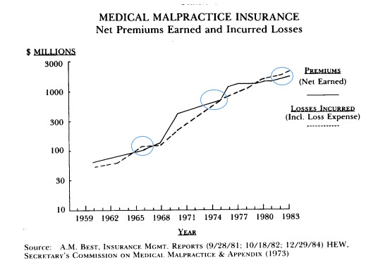
The oldest evidence of the MedMal cycle I could find is the following exhibit from the study by James Posner (Posner 1986) that reveals there was a period when losses exceeded premium in the mid-1960s. The circled time periods in Figure 3.1.1 are when losses exceeded premiums. This chart shows losses in the mid-1960s, mid 1970s and early to mid-1980s.

It is well documented that there was a MedMal insurance crisis in the mid-1970s. According to Posner, “The cost of a constant level of medical malpractice insurance coverage increased seven-fold for physicians, ten-fold for surgeons, and five-fold for hospitals between 1960 and 1972. Many factors contributed to the mid-1970s malpractice crisis….” (Posner 1986)

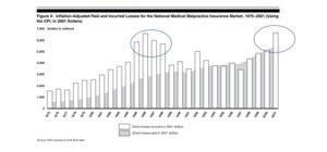
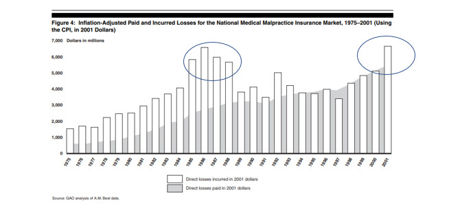
The following graph is from the 2003 GAO report (United States General Accounting Office 2003).

When this graph was published, the industry was just entering the MedMal crisis of the early 2000s. The circled time periods in Figure 3.1.2 show the MedMal crisis time periods. These crisis periods coincide with the jump in Direct Losses incurred adjusted for CPI economic trend as shown in the graph.

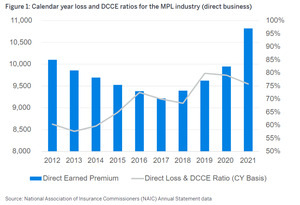
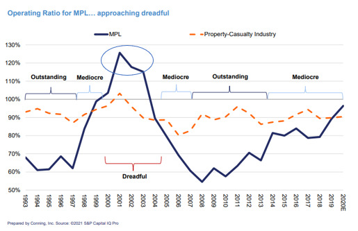
To illustrate the time period subsequent to the GAO study, a recent Conning Market presentation (Conning 2021) graphic shows the full crisis in the early 2000s and how the current market appears to be entering another period of higher losses.

These 2 prior graphs illustrate that there were industry losses in 1985, a “dreadful” period around 2001, and another starting in 2019.

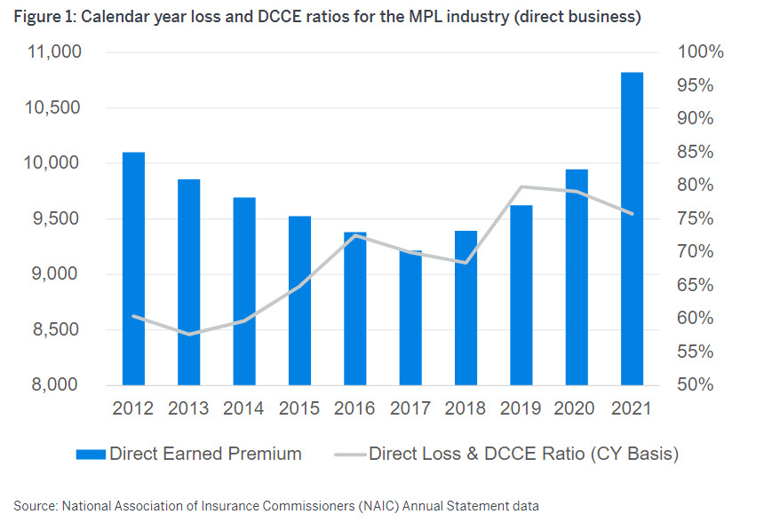
Subsequent to 2019, the Covid pandemic created an unusual situation with regards to MedMal claims. With the courts closed, there were few if any cases brought to court. There were also settlements that may not normally have happened except for the COVID shutdown. So COVID is an external event that has affected the normal trend patterns. Results in 2019 and 2020 show some improvement over prior years due to this “Key Event” as illustrated in the following graphic from a presentation by Vega (Vanderpool 2022).

Various publications allude to the fact that these historic crises included a jump in severity as seen in the following quotes:

• NAIC study (Sowka 1981) after 1975 crisis –

  • “Between 1975 and 1978, the average award per injury increased 70%”.

  • “A major factor contributing to the growth of indemnity was the increase in large settlements or judgements.”

  • “Prior to 1975, only 5 awards of $1M or more were reported…in 1978, 23 paid claims equaled or surpassed $1M.”

• Mid 1980s crisis - “St. Paul reports that paid claim severity increased ninety-five percent during the five-year period 1979-1983, from $27,408 in 1979 to $53,482 in 1983”. (GAO report on premium increases [United States General Accounting Office 2003])

• The average malpractice jury award is reported to have risen from $404,726 in 1980 to $954,858 in 1984. (GAO report on premium increases [United States General Accounting Office 2003])

• In 2002, Conning released an extensive report that found that the medical malpractice insurance market had deteriorated rapidly for several reasons including “rapidly deteriorating loss ratios as a result of dramatically increasing severity.” (Conning and Company 2001)

So, there were noticeable “crisis” periods in 1965, 1975, 1986, and 2000 the last three all of which were accompanied by an increase in claim severity. The current severity jump we are seeing started to appear again beginning in CY 2016. It is this repetitive pattern of crises every 10 to 15 years that is key to the model being proposed.

3.2. Jury Verdict Data

As the MedMal insurance arena hit crisis mode in 2001, insurers scrambled to try to make sense of what was happening and how to fix it. Actuarial Standard of Practice No. 13 defines social inflation as “the impact on insurance costs of societal changes such as changes in claim consciousness, court practices, and legal precedents, as well as in other non-economic factors.” (Actuarial Standard of Practice No. 13, Trending Procedures in Property/Casualty Insurance Ratemaking 2009) In line with this definition, many insurers pointed to jury verdict research data to explain the increase in severity being observed. The table below shows the data available from Jury Verdict Reporter (JVR) (Jury Verdict Research 2005) at the time. Figure 3.2.1 shows that after about 5 years of relatively flat median severity, between 1993 and 1997, the median climbed quickly to double the level it used to be between 1998 and 2000. This was a sign that social inflation was on the rise for MedMal at that time.

Graphically, looking at the median jury verdict, it is easy to see that the median verdict took a bigger than expected jump after 1997.

Figure 3.2.2 shows how the median jury verdict was fairly level up to 1997 (2% trend) then doubled in just 3 years – from about $500K in 1997 to $1M in 2000. The median settlement value in the JVR database mirrors the median verdict in that settlement levels doubled between 1998 and 2002. This relationship between the median verdict and the median settlement is consistent with observations by claims personnel that as jury awards go up for specific injuries, settlement request levels follow suit. Note that the median gives a measure of how the whole distribution of claims is moving. The mean can be affected by one very large verdict. The JVR data was the first hint that something was going on with claim severity to trigger the crisis.

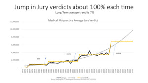
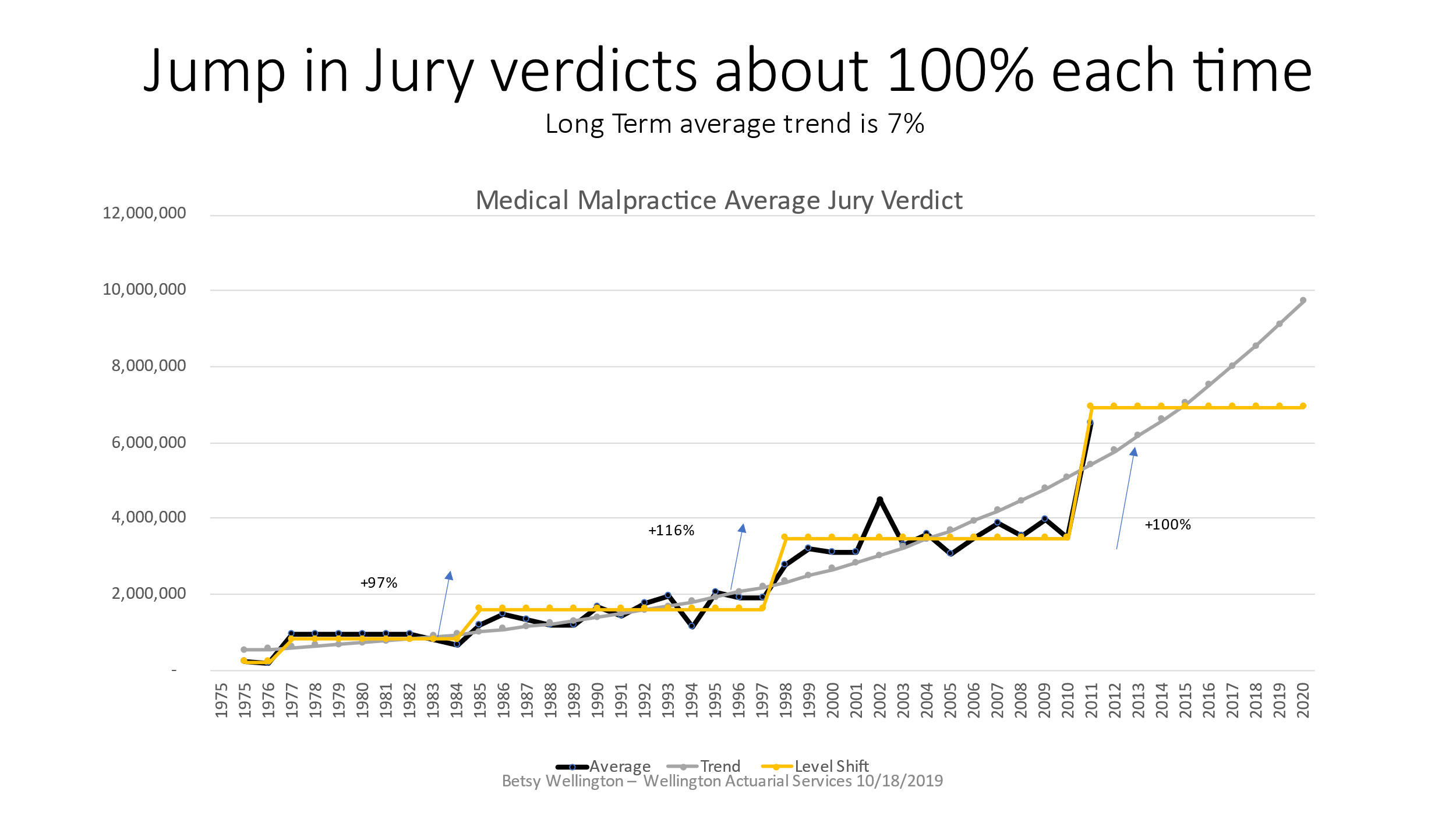
JVR stopped publishing the MedMal jury verdict data after 2010. As shown in the next graphic, Figure 3.2.3 shows the average MedMal jury verdict for the full period of time that information could be found via JVR’s publications and news releases. The graph illustrates that when the jury verdict averages jump up, they tend to double in value. In addition, after the jumps occur, there appears to be a leveling off of the severity. Looking at the averages over this longer period of time shows a stair step pattern in which the severity shifts up to a new level that plateaus rather than continuing at a constant rate of change. The median was not available over this longer time period. It should be noted that these level shifts also fall into the same cycle range as our MedMal crises – every 10-15 years.

Statistically, the mean absolute error of the exponential trend is $451K versus that for a level shift fit which is $260K resulting in a 42% reduction in error demonstrating a better fit. Of course, the big question is whether or not the projection of a level shift in 2011 will continue or not. In 2003, based on the data from Figure 3.2.1, I had projected the jury verdicts to flatten out which is exactly what happened if you examine the above graph. JVR stopped publishing this information in 2010 so this particular source cannot be continued. This graph will be revisited in section 7 to reveal what happened after this time period.

3.3. Insurance Claim Data

One criticism used against the JVR data is that it represents jury verdicts rather than actual insurance settlement payouts. In order to see what is happening with insurance payments on MedMal cases, the National Practitioner Data Bank (NPDB) public use file (National Practitioner Data Bank Public Use Data File, [12/31/2021], U.S. Department of Health and Human Services, Health Resources and Services Administration, Bureau of Health Workforce, Division of Practitioner Data Bank. 2021) can be used to calculate average indemnity payments by calendar year by state as well as develop the ultimate paid severity by AY. It is important to analyze this line of business by state, if possible, because there are significant differences between MedMal laws by jurisdiction. When using the NPDB data it is important to keep in mind the following facts:

1. NPDB is publicly available data.

2. Data is indemnity payments only.

3. Payments are made against individual practitioners only – no hospital or corporation data is included.

4. I have excluded any payments other than those against physician and surgeon related classes since other classes reported are not compulsory.

5. All payments made on behalf of physicians and surgeons must be reported irrespective of who their employer is or whether they are self-insured or covered by some form of insurance.

6. Insurance companies under receivership can distort the data.

7. Batch claims can affect the averages, so adjustment is needed.

8. Claims in fund states must be accumulated into occurrences.

9. Compliance may not be 100%.

Please refer to American Academy of Actuaries publication “Important Considerations When Analyzing Medical Malpractice Closed-Claim Databases” for more information (Important Considerations When Analyzing Medical Malpractice Insurance Closed-Claim Databases, Medical Malpractice Subcommittee 2005). The use of any database requires proper due diligence, and I suggest that anyone using this data refer to the notes included with the downloads to make any necessary adjustments before using the data for analytics.

When I first reviewed the NPDB data in 2001, it was clear that there was a jump in paid severity around CY 2000 across the country. The severity level shifts happen at slightly different times from year to year in different states. But 1999/2000 showed an unusual pattern of almost every state having a large increase in the payment severity over the prior year. The three subsequent years reverted back to the prior pattern of smaller up and down changes, however they bounce around a higher severity level than pre 1999/2000. I refer to this jump in severity as a Level Shift because the severity jumps to a new level and then the average severity stays at this new higher level for a number of years.

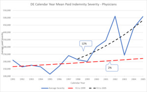
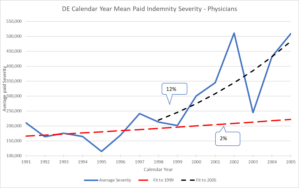
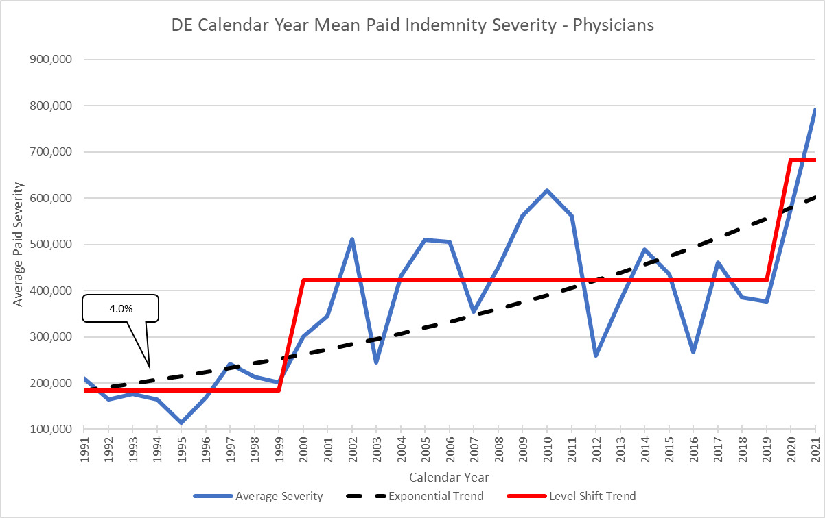
As an example, back in 2005 Delaware exhibited the pattern shown in Figure 3.3.1 that reveals a severe increase in severity starting in 1999. Although DE is a small state, there were no significant events such as tort reforms in the state and there are no significantly different jurisdiction differences within the state. So, although small, DE is relatively homogeneous. Similar to the JVR data, fitting an exponential trend line up to the point prior to the jump in 1999 and subsequent to this jump results in very different trend indications.

On a CY basis, 1991-1999 are fairly flat (2%), which is similar to the JVR jury verdict data. Then between 2000 and 2002, there is a steep increase in trend to 12% which is also similar to the JVR data. As actuaries we must figure out what the trend will be on a going forward basis while being told by underwriters that this jump in severity is a “one off” situation. This could be the case in DE because there is a new high maximum paid claim of $13M in the state in 2002. This is another statistic that can be tracked using the NPDB data. A new maximum can be a very early warning that some sort of jump may be on the horizon. In this case, by doing additional research on the jurisdiction and analytics on the data, it is possible to project that this is actually a level shift to a new higher level of severity for the state and not a “one off” claim. That very large payment was actually a harbinger of average severity moving up.

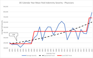
Here is the updated graphic for DE that clearly shows the Level Shift to a new average base:

Clearly the jump starting in 1999 was a move to a new level of average severity. Note how it did not continue to increase exponentially but rather leveled out to a similar stair step pattern that we saw in the jury verdict data. The long-term average exponential trend for this time period is 4% which incorporates a full trend cycle of 20 years. Delaware is just one example but level shifts like this are found in almost all states. The specific timing and magnitude of the jump and the long-term exponential trend differ by state so should be examined separately.^[1]

4. CALENDAR YEAR TREND MODEL

The prior sections demonstrate how jury verdicts and insurance payment severity show a stair step pattern when looked at on a CY paid basis. The relationship between the two indicates that this jump is largely due to social inflation as defined by the American Academy of Actuaries (AAA). In the absence of some other catalyst, it is reasonable to assume that general social inflation is causing the jump in severity when tracked back to a jump in jury verdicts.

If severity trend behaves in a stair step pattern on a calendar year paid basis, how can this be used in actuarial pricing of medical malpractice policies or reinsurance treaties? The easiest way to incorporate this in the pricing model is to create trend factors that properly reflect this recurring pattern. These trend factors can be used for on-leveling historic losses as well as for projecting future loss levels.

4.1. Current Trending Method

Traditionally, actuaries use a report year, accident year or policy year-based approach to analyze severity trends for MedMal. These methods all involve using development techniques or methods to estimate outstanding reserves before calculating trend factors. Using a CY Paid approach completely removes the uncertainty of development techniques. Werner notes in “Basic Ratemaking,” “if calendar year data is used to measure loss trend, one of the underlying assumptions is that the book of business is not significantly increasing or decreasing in size. This assumption sometimes does not hold in reality and therefore using calendar year data to measure trend can cause over or underestimation of the trend. The problem with calendar year data is that claims (or losses) in any calendar year may have come from older accident years, yet they are matched to the most recent calendar year exposures (or claims). A change in exposure levels changes the distribution of each calendar year’s claims by accident year.” (Werner and Modlin 2010) The benefit of using the NPDB is that it is the complete population of all cases against physicians so it is unlikely that there will be shifts in exposures that would affect the CY severity. As long as the demographic mix of the population that might lead to smaller or larger severity cases did not change significantly, the average severity should not be affected by changes in volume of population within the state. An example of a change in mix of demographics that might affect CY severity is if the birth rate changed disproportionately to population. Birth claims are very high severity so a big shift in this exposure could cause the CY severity to change. That being said, actuaries should use all standard techniques for aligning exposures and losses using the CY method that they would use on other methods. It is also possible that changes in claims settlement patterns might artificially change the CY severity in a single year so this should be part of the actuarial review as well.

Another issue that is problematic with the standard trend approach is that actuaries will frequently use shorter time periods for determining going forward trend factors in order to be more responsive to recent trends. For example, a long-term report year indicated trend using 10 years of data may indicate a 7% trend while the last 4 years may only indicate 3%. The actuary may then use their judgment to select 3% going forward and discount the larger trends from the past. Under a level shift situation in which the severity jumped 10 years ago and then leveled out, using a method of shorter time period indications will produce a cyclical trend. So closer to 10 years ago, the selection would be greater than 7% whereas more recently it is only 3%. These estimates are lagged RY or AY trend indications and will always be behind the actual cycle.

4.2. Level Shift Trending Method

The following proposed model incorporates the observed level shifts and long-term trends into a model that will coincide with the cycle rather than being lagged from the cycle. The method will be demonstrated using an example.

Some simplifying assumptions used in order to make the example easy to follow are:

• All policies incept 1/1.

• Data is homogeneous.

• Severity jump occurs at the beginning of the year and affects all losses paid in that year equally.

• There is no frequency trend.

• Level Shifts are cyclical – they repeat.

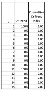
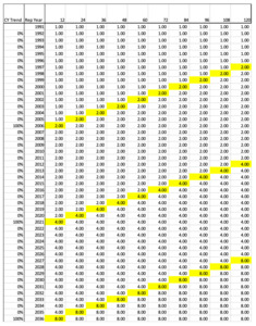
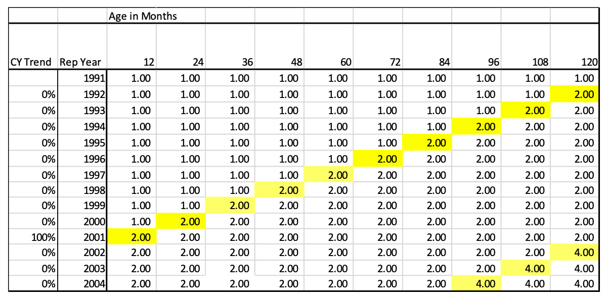
For the first example illustrated in Figure 4.2.1, a cumulative calendar year trend index is created that assumes the paid severity has a repeating cycle of flat severity for 9 years and then a level shift jump of 100% in the 10th year (the equivalent of severity doubling in value). The CY trend is the nominal change in year i. The cumulative trend is calculated starting with i=1. The initial year should be set to 1.0 to normalize the calculations. So, our model is showing a case where the CY severity doubles every 10 years.

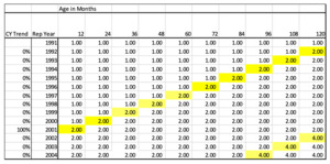
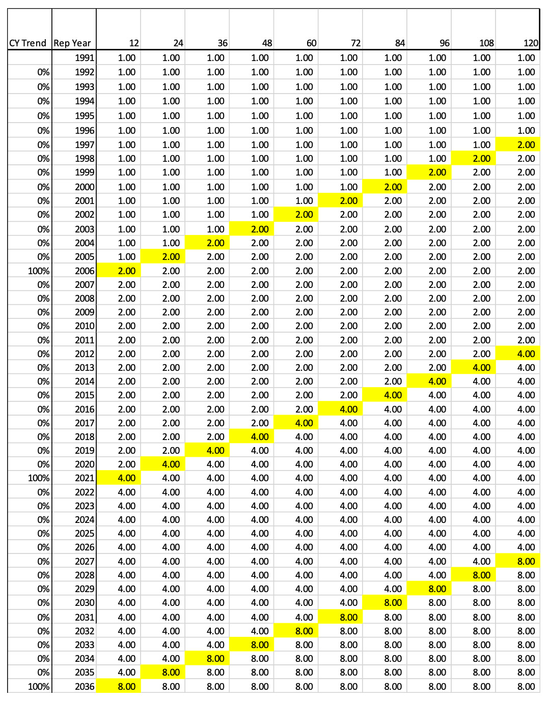
Since claims made policies are rated on a RY basis, this CY index needs to be converted to a RY trend index. To do this, the cumulative normalized trend indices for each calendar year get allocated to the appropriate report year by development age. Figure 4.2.2 shows the allocation of these CY indices to the Report Year by Age.

This pattern can be interpreted as claims that are reported in 2000 and paid in 2000 (age 12), will be paid at a rate of 1.0 whereas claims reported in 2001 and paid in 2001 (age 12) will be paid at a relative rate of 2.0 just due to the jump in severity that occurred in CY 2001. This also means that claims reported in 2000 but paid between 2001 and 2010 (ages 24-120) will be paid at a relative rate of 2.0 times those paid in 2000 at age 12.

To square or fill the triangle, a repeating pattern of future jumps is assumed. In this example, we assume there is a level shift every 10 years. This would mean a second jump occurs in CY 2011 and then another is CY 2021. The assumption that the cycle repeats at a certain number of years is key to using this model. This assumption will be addressed in section 4.4. So, to continue to complete the matrix, we assume that another 100% Level Shift will happen in an additional 10 years. For example, look at Report Year (RY) 2004 at age 96. At this point another level shift is projected to occur in CY 2011 that is equal to the magnitude of the prior jump, so it doubles again. Thus, the accumulated factor is (1+100%)² = 4.0.

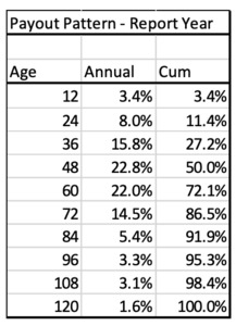
In order to calculate the actual RY trend factors, a relative ultimate cost index for each report year is calculated. This can be done by using the report year payment pattern to create a weighted average annual cost index. Occurrence policy trend factors are calculated using an accident year payment pattern. The following example uses a 10-year Report Year payment pattern as follows:

To calculate the ultimate index, the annual payout percent is multiplied by the Report Year indices shown below:

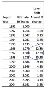
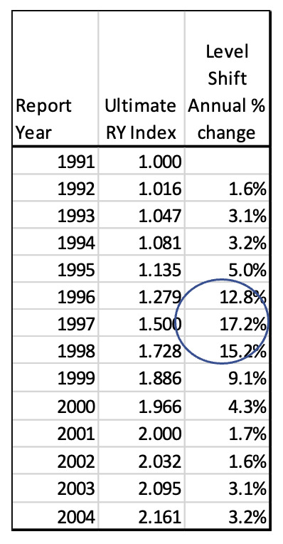
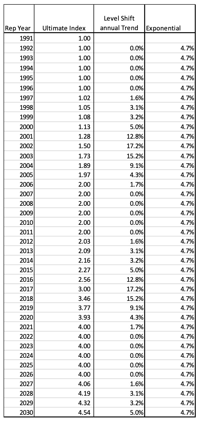
The Ultimate Report Year 1995 index is equal to the sum of all the individual age weighted annual payment values. The Total RY index is the sum of the age 12 through age 120 Annual CY Contributions in this example. The Ultimate index for 1995 is 1.135 rather than 1.00 due to the level shift in severity that happens in CY 2001, which is age 84 for RY 1995. So, on average the ultimate severity for 1995 claims will be 13.5% more than for 1991 claims.

To calculate the final trend factors, these RY Ultimate indices are calculated for each year and then the annual rate of change is calculated.

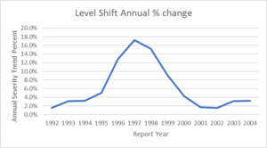
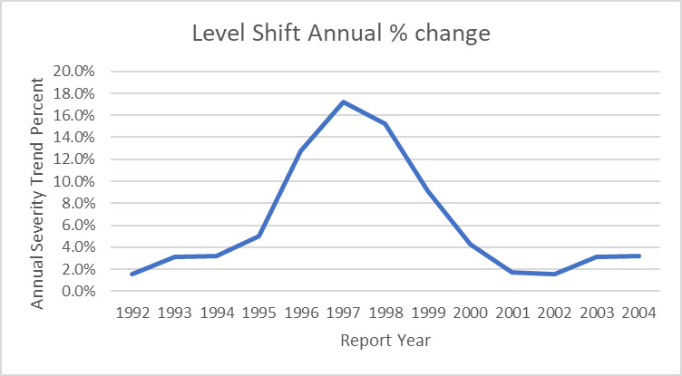
Note how the largest trend factors occur 4-5 report years BEFORE the level shift. This is because the largest portion of an individual report year’s claims are paid 4-5 years after the report year. This is a big driver of adverse development on the MedMal line. Below is the graphic of the cycle of trend factors for this model:

4.3. Level Shift Trending Method Mathematics

Mathematically, start with the CY severity Level Shift vector which has 9 years of 0% and 1 year of 100%.

1. Vector u = The CY Trend annual percent change from Figure 4.2.1 column 2

$$\mathbf{u}=[0 \%, 0 \%, 0 \%, 0 \%, 0 \%, 0 \%, 0 \%, 0 \%, 0 \%, 100 \%]$$

2. i = report year or accident year or policy year

3. Create a cumulative CY index vector c from Figure 4.2.1 column 3, where:

$$\begin{gathered} \mathbf{c}_1=1 \\ \mathbf{c}_{\mathrm{i}+1}=\mathbf{c}_{\mathrm{i}} *\left(1+\mathbf{u}_{\mathrm{i}+1}\right) \\ \mathbf{c}=[1.0,1.0,1.0,1.0,1.0,1.0,1.0,1.0,1.0,2.0] \end{gathered}$$

Create the payout matrix A using the accumulated indices calculated above. The matrix will have the following general form.

$$A=\begin{bmatrix} c1 & c2 & c3 & c4 & c5 & c6 & c7 & c8 & c9 & c10 \\ c2 & c3 & c4 & c5 & c6 & c7 & c8 & c9 & c10 & c11 \\ c3 & c4 & c5 & c6 & c7 & c8 & c9 & c10 & c11 & c12 \\ c4 & c5 & c6 & c7 & c8 & c9 & c10 & c11 & c12 & c13 \\ c5 & c6 & c7 & c8 & c9 & c10 & c11 & c12 & c13 & c14 \\ \end{bmatrix}$$

To model the previous example, namely a 100% severity jump every ten years and a report year that is completely paid out over ten years, the matrix A corresponding to the relative rates in Figure 4.2.2 looks like this:

$$A=\begin{bmatrix} 1.0 & 1.0 & 1.0 & 1.0 & 1.0 & 1.0 & 1.0 & 1.0 & 1.0 & 2.0 \\ 1.0 & 1.0 & 1.0 & 1.0 & 1.0 & 1.0 & 1.0 & 1.0 & 2.0 & 2.0 \\ 1.0 & 1.0 & 1.0 & 1.0 & 1.0 & 1.0 & 1.0 & 2.0 & 2.0 & 2.0 \\ 1.0 & 1.0 & 1.0 & 1.0 & 1.0 & 1.0 & 2.0 & 2.0 & 2.0 & 2.0 \\ 1.0 & 1.0 & 1.0 & 1.0 & 1.0 & 2.0 & 2.0 & 2.0 & 2.0 & 2.0 \\ 1.0 & 1.0 & 1.0 & 1.0 & 2.0 & 2.0 & 2.0 & 2.0 & 2.0 & 2.0 \\ 1.0 & 1.0 & 1.0 & 2.0 & 2.0 & 2.0 & 2.0 & 2.0 & 2.0 & 2.0 \\ 1.0 & 1.0 & 2.0 & 2.0 & 2.0 & 2.0 & 2.0 & 2.0 & 2.0 & 2.0 \\ 1.0 & 2.0 & 2.0 & 2.0 & 2.0 & 2.0 & 2.0 & 2.0 & 2.0 & 2.0 \\ 2.0 & 2.0 & 2.0 & 2.0 & 2.0 & 2.0 & 2.0 & 2.0 & 2.0 & 4.0 \\ 2.0 & 2.0 & 2.0 & 2.0 & 2.0 & 2.0 & 2.0 & 2.0 & 4.0 & 4.0 \\ \end{bmatrix}$$

This matrix represents any 11-year period (11 rows). It has 10 columns because of the 10-year payout pattern. If the payout pattern is longer, then additional columns can be added. To model a 75% jump every 8 years, the first row would change to seven 1.0’s followed by three 1.75’s. In the new pattern, the 4.0’s would be in different locations and would change to 1.75² = 3.0625.

Next create a vector r that represents the RY annual percent payout pattern. For this example, using the numbers in Figure 4.2.4 and converting percentages to decimals,

$$\mathbf{r} = [.034 .080 .158 .228 .220 .145 .054 .033 .031 .016]^{\text{T}}$$

(^T means transpose)

Taking the matrix A times the vector r gives a vector p containing the Ultimate index for each year which corresponds to the Ultimate Report year Index of Figure 4.2.5:

$$\mathbf{p} = A\mathbf{r} = [1.000 1.016 1.047 1.081 1.135 1.279 1.500 1.728 .1886 1.966 2.000]^\text{T}$$

The ith entry of the vector p is:

$$\mathbf{p}_{i} = \sum_{j = 1}^{10}{A_{i,j}r_{j}}\tag{4.3.1}$$

Finally, the annual trend factors are

$$\frac{\mathbf{p}_{i}}{\mathbf{p}_{i - 1}} - 1\tag{4.3.2}$$

4.4. Calculating the Expected Length of Cycle

The expected length of the Level Shift cycle, y, can be solved for as a function of two actuarially determined parameters, 1) the expected long term exponential trend, t, and 2) the magnitude of the Level Shift, m. The relationship between these variables can be thought of as similar to a simple compound interest calculation where we want to solve for how long it will take to increase an investment by m % at an interest rate of t. These variables are related by the equation

$$(1 + t)^{y} = 1 + m\ \tag{4.4.1}$$

Solving for y gives

$$y = \frac{\ln{(1 + m)}}{\ln(1 + t)}\tag{4.4.2}$$

For example, if the long-term exponential trend is 5% and the severity of the level shift is 100% (the severity doubles), the cycle will be calculated as

$$y = \frac{\ln{(1 + 1.00)}}{\ln(1 + .05)} \approx 14.2$$

Thus, the case of a long-term annual trend of 5% compared to the case of an annual trend of 0% coupled with a jump of 100% every 14.2 years will end up in the same place at the end of the cycle. The assumption is that the social inflation level shift is cyclical and happens on a continuing repeating basis. Real data reveals that this is a reasonable assumption although the jumps might not occur on an exact annual point estimate but perhaps over 2 or 3 years. For simplicity, a specific year point estimate is assumed for the Level Shift.

4.5. Calculating the Exponential Equivalent to Level Shift

Equation 4.4.1 can also be used to calculate the underlying long term exponential trend, t, given a level jump magnitude, m, and an estimate of how often this happens, y. A review of historic data may show that the severity jumps 100% every 10 years. Thus,

$$t = \sqrt[y]{1 + m} - 1 = \sqrt[10]{1 + 1.00} - 1 \approx 7.18\%$$

Therefore, for this example, the underlying long term exponential trend is 7.18%.

4.6. Example: Exponential Trend Comparison to Cyclical Level Shift Trend

So how does the simple constant exponential trend method compare to the Level Shift method? It can be shown that the Level Shift method gives equivalent results as using an exponential trend method but instead of annual equal jumps, the Level Shift has one large jump over the time period it would take to accumulate the exponential annual trends to the same magnitude.

All the above math can be used but now assume that the rate of change by year is a constant 7.2% rather than 0% followed by a jump.

Using the annual trend rate of 7.2%, matrix A now looks like this:

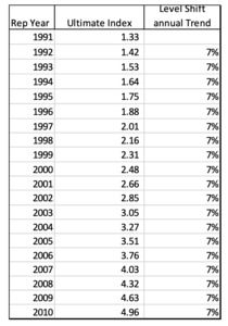
This matrix shows how the year of the level shift in CY 2001 has the same cumulative trend factor (2.0) as the equivalent annual exponential trend factor of 7.2%. Note that the vector u has the same 7.2% annual percent change for each year instead of the 0% s and 100% which is the equivalent of a 7.2% exponential trend.

Using the same index calculation weighted by the same payout pattern gives us the following ultimate cost indices by report year which results in the original implied annual exponential trend rate of 7.2%.

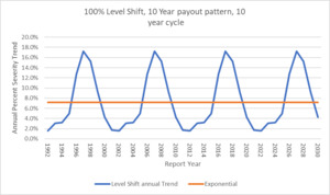
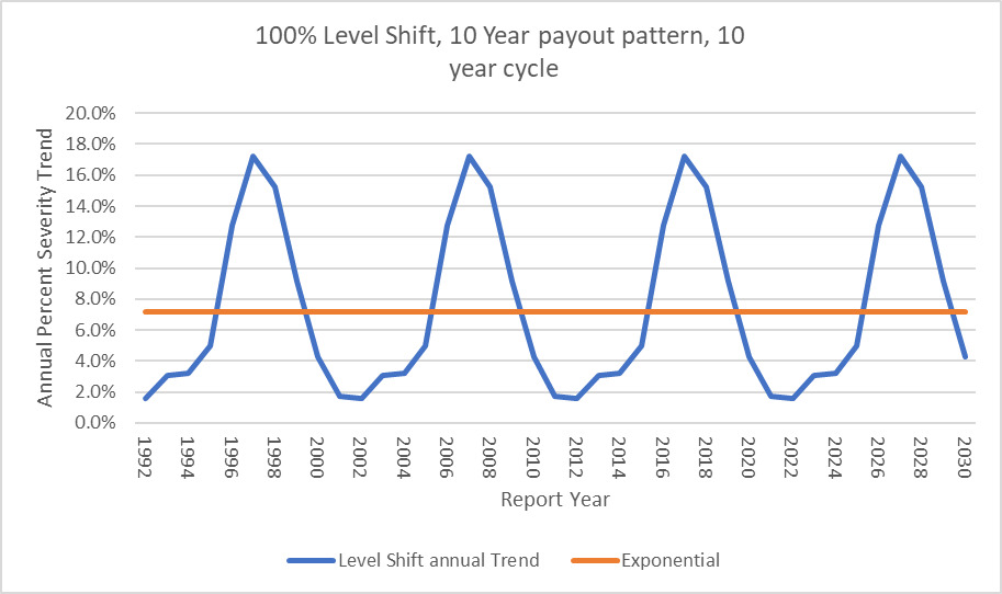
The following illustration shows how the level shift method results in a cyclical trend factor versus the flat annual exponential trend but they both average out to the same point estimate long term trend of 7.2%.

Now instead of a single annual constant trend factor to use going forward, the model produces a cyclical trend index that can be used. This graphic has the trend extended to RY 2030 by assuming the repeating pattern of 9 years of flat 0% trend followed by a jump of 100%.

4.7. Economic Inflation

Now that the model has been shown to be able to accommodate both a Level Shift every year such as with the exponential model or a Level Shift every number of years due to social inflation, it is easy to see how economic inflation could also be incorporated in the model. If there is an economic inflation index that is appropriate for MedMal in the state being examined, that index could be used in the individual years and then the Level Shift incorporated in the appropriate time periods. So, the vector u would look something like this assuming constant 2% inflation in non-social inflation years.

$$\mathbf{u}=[2 \%, 2 \%, 2 \%, 2 \%, 2 \%, 2 \%, 2 \%, 2 \%, 2 \%, 100 \%]$$

Incorporating economic trend based on an external index is possible but should be studied carefully compared to actual MedMal data to make sure that there is a good correlation between the economic index and actual insurance data. Similar to social inflation, I would expect economic inflation to affect MedMal claims on a CY basis which means it will affect all open claims.

4.8. Estimating Level Shift Parameters

The two essential input parameters to the Level Shift model are:

1. the expected magnitude of severity jump, and

2. the long-term exponential severity trend.

To estimate the expected level of the jump, it is necessary to use a long time period of loss data. To estimate where there is a level shift, a piecewise exponential model could be used to fit multi-year segments. Another method is to examine the data and look for the point where severity no longer goes up and down around an average. The severity history should also be mapped against known events in the jurisdiction that might move the severity in order to help identify pivot points. Another indicator to look at is the maximum paid claim to see if it has moved to a higher level. Precedent setting jury verdicts may also indicate that there is a level shift. Just like any actuarial analysis, appropriate data should be gathered, and sound actuarial judgment and assumptions can be used to estimate the historic jumps.

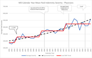
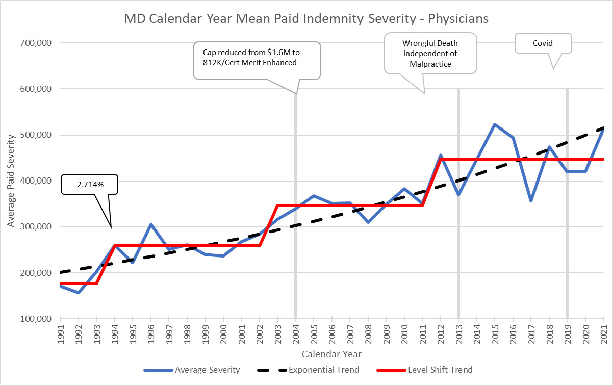
Here is another example using Maryland which has level shifts of around 30% when it jumps. In addition, I have added some call outs showing events that might contribute to severity changes. This state has an adjustable but large cap on pain and suffering which limits the magnitude of the potential jumps. Comparing MD to DE with very different magnitudes of Level Shifts illustrates why the analysis needs to be done separately by jurisdiction.

Typically, there will only be 3 or 4 data points available with which to evaluate the magnitude of the jump. This lack of significant data for an individual state might cause concerns about credibility. I have two comments about this issue. One is that in my experience, MedMal data has a lot more credibility to small amounts of data, as long as you have a very long history, than standard credibility models might suggest. Second, when you review the patterns of 50 different states, you can see that they tend to fall into 3 categories of magnitude jump – 25%, 50% and 100%. These jumps are related to the length of the payout pattern where those with longer tails tend to have longer cycles and bigger jumps, as well as tort reforms in place and policy limit capping. Therefore, there are more considerations that can be used to help make this estimate for any one state. But like any actuarial parameter selection, it is necessary to consider all data available and make reasonable judgment calls.

To estimate the long-term exponential trend, the analysis must reflect the full MedMal cycle. As shown earlier, MedMal has a 10 to 15-year cycle depending on the jurisdiction. This implies that a long history of data is required to properly estimate the long-term exponential trend. A trend analysis of calendar year paid data should balance to the same long term exponential trend as a report year or accident year-based analysis. It is important to see that those two methods result in trend indications in the same ballpark for the analysis of the long-term trend to make sure nothing is being missed.

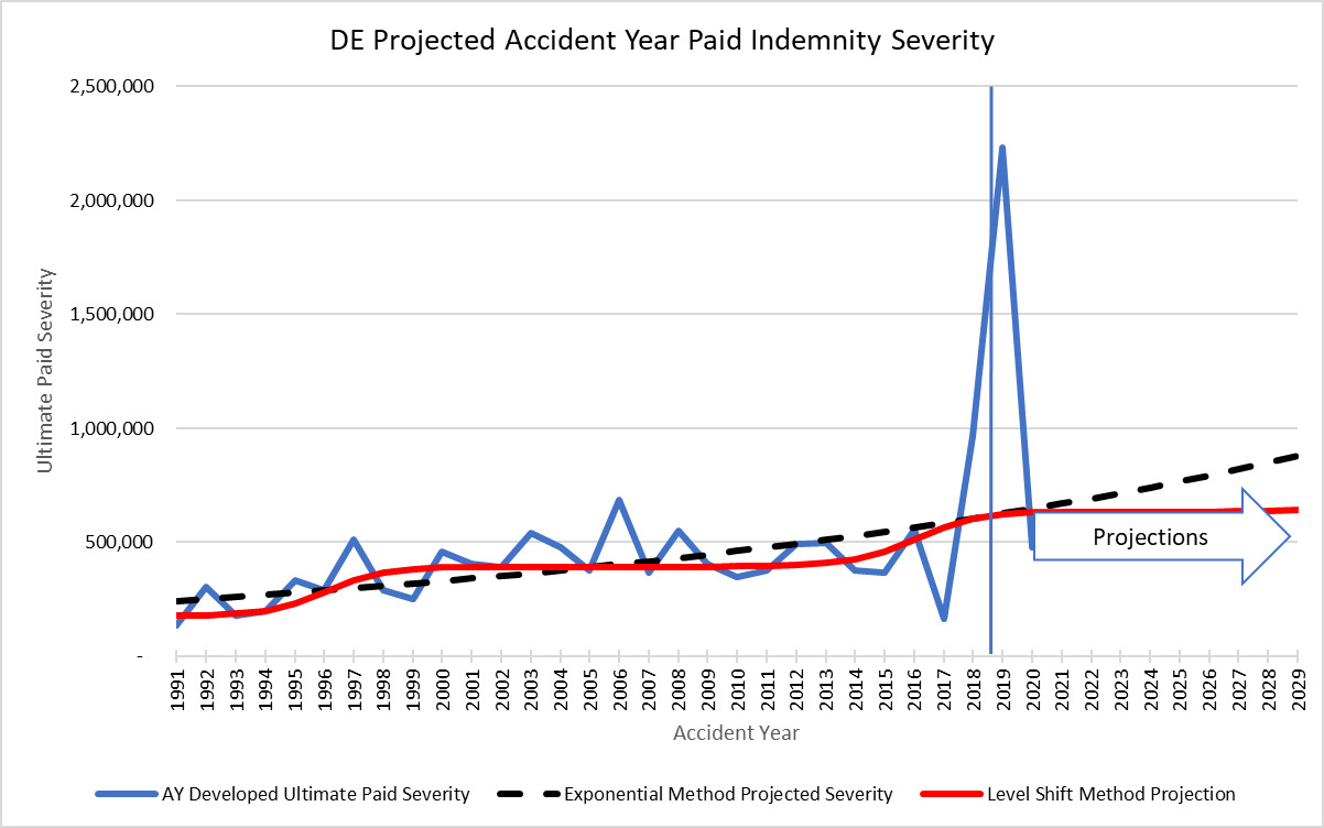
The above graph shows an example of the comparison of accident year ultimate trends to the calendar year level shift trends. It shows how the AY paid development has a lot of uncertainty to the projections in the most recent years, but the CY method does a good job of reflecting the cycle. In this case, the AY exponential trend is 3.4% with a lot of uncertainty versus the CY exponential of 3.8%.

5.0. Why Use the Level Shift Model

If the Level Shift and exponential models have the same long-term trend result, how can the Level Shift model help in pricing and reserving analyses? In order to assess how this model can help, it is important to examine what actually happens with pricing and reserving when looking at a line of business where there is a cyclical trend.

5.1. Level Shift compared to Standard Insurance Services Office (ISO) Trend Method – Number of Years used for Averages

Let’s start with how ISO determines projected trend factors for MedMal. The only parts of the ISO method to be addressed are 1) ISO uses indicators that range from a 6-year to 8-year average and 2) ISO presents factors based on both Incurred Loss and Paid Loss RY, AY and PY methods. ISO is used to represent standard industry methods.

The 6-year period would be considered more responsive to current levels and the 8-year trend would be for the longer term. However, if MedMal has a 15-year severity trend cycle how would the ISO method be expected to play out?

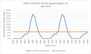
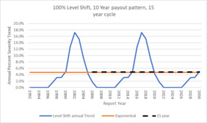
To illustrate what would be expected to be seen, we will use an example of the Level Shift method where the ultimate Report Year indices assume an underlying pattern of 100% severity jump every 15 years. The long-term underlying exponential trend associated with these parameters is expected to be about 4.7% using Equation 4.4.1.

$$t = \sqrt[y]{1 + m} - 1 = \sqrt[15]{1 + 1.00} - 1 \approx 4.7\%$$

In this case, the matrix A will be extended substantially.

Using the same 10-year payout pattern, the ultimate RY Trend indices on a level shift and an exponential basis are now:

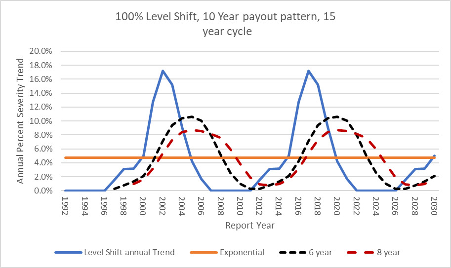
The following graph illustrates the cyclical pattern with underlying long-term trend of 4.7%:

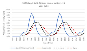
If this is how trend is moving, then how does the ISO method compare? The curves shown below in Figure 5.1.4 represent 6-year and 8-year moving average trend factors based on the Level Shift Indices. These results indicate that taking an average of a number of years that are shorter than the actual cycle will assure that the indications are behind the times. When the Level Shift method shows that the 2016 RY will have a 17% trend, the standard methodology will only be between 6% and 8%. But when the real trend starts going down, the ISO method is going up to its peak (2020). This lag is why the industry is shocked when a Level Shift occurs. The severity jump affects the prior Report Years which is the cause of adverse development.

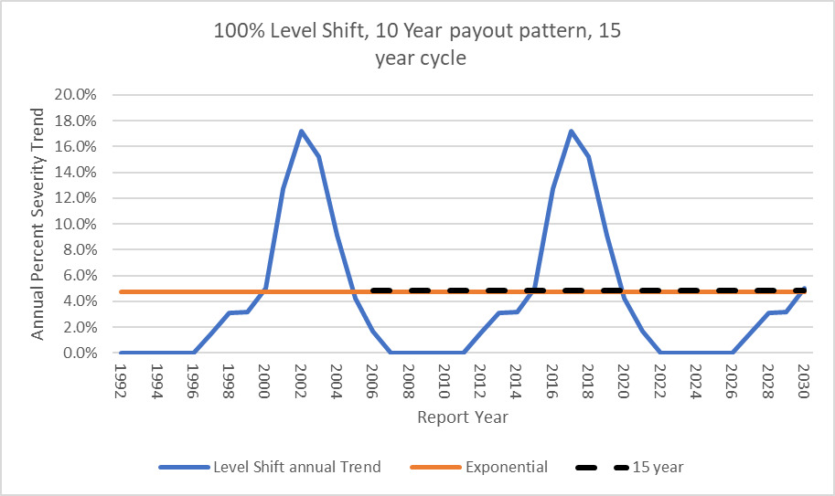
For comparison, using the standard ISO methodology and a 15-year average, which is the length of the cycle in this example, the ISO method exactly matches the long-term underlying exponential trend.

By using the cyclical Level Shift trend method, actuaries can be much more responsive to current events including social inflation than when using standard trending methods.

5.2. Level Shift compared to Standard Insurance Services Office (ISO) Trend Method – Using Paid vs. Incurred

The second standard trend analysis element to be addressed is the difference between using a paid method and an incurred method for MedMal. As discussed previously, the ultimate value of an individual MedMal claim is determined by the year in which it is paid and not a function of the report year or accident year. Standard actuarial methods for determining trend factors involve developing losses and claim counts to ultimate on a paid or incurred basis by report year, accident year or policy year. In these methods, any calendar year effect is supposed to be picked up through the development factors. In addition, actuaries will typically use incurred development because there is more data available than for paid development.

When using an incurred development method, the following question needs to be addressed. If there is a jump in severity, how do case reserves respond? This is a question for the claim adjusters. Discussion with claims experts indicates that with respect to open claims, claims departments do NOT respond to the evidence that settlement values are increasing due to social inflation. They do not go back and adjust open reserves upwards unless there is an imminent settlement coming up. They might set up reserves on newly reported claims at a higher level, but they will not adjust all open claims. Therefore, what would be expected to be seen in the incurred development triangles if this is the case?

If the claims adjusters are not adjusting historic open claims for the expected jump in severity, then we would necessarily see adverse development in our incurred loss development triangles. We would also see the indicated trend factors based on incurred development to be LOWER when this jump occurs than for a paid development method. The paid claims are showing the higher severity of settlements whereas the incurred claims only reflect this higher severity to the degree that the claims have been paid. Since there are virtually no partial payments in MedMal, this means that the Incurred claims are understated when there is a jump in severity. Actuaries tend to discount the paid method due to the lower credibility of less data than for the incurred. As claims get paid at the higher severity level, then the trend indications for incurreds will be expected to start to catch up with the paid claims. The incurred trend indications are more delayed to show the jump than the paid indications. On a paid development basis, we would expect to see adverse development just because severity has increased. However, with the thinner data for paids, it is always difficult to give the higher LDFs the credibility and weight that they deserve. For MedMal, it is important to do both paid and incurred indications and then make sure they balance. If they do not balance, then further analysis should be done to figure out why.

The conclusion of this discussion is that standard actuarial methods will be very biased upwards or downwards depending on the point of the cycle we are in if the underlying loss severity pattern is cyclical in nature as described in the introduction. Shatoff explains the details of this situation in his paper “Loss Reserving and Ratemaking in an Inflationary Environment.” (Shatoff 1981) I recommend this paper for further study of this phenomenon.

6.0. QUANTIFYING THE EFFECTS OF EXTERNAL KEY EVENTS

I have spoken about general trend which can reflect a combination of economic factors and social inflation. The model developed above can also be used to quantify the expected effect of external events that will move the loss costs for MedMal. The most relevant external event for MedMal is changes in Tort Law in a state. I will use Texas as an example and data from the NPDB to show how the Level Shift method can be used to project severity and frequency levels.

6.1. Example: Effect of Tort Reform

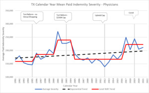
In 2003, Texas implemented a constitutional change that limits pain and suffering payouts on medical malpractice claims to $250,000. The Paik paper quantified the effect of the tort reform to be a 35% reduction in severity and a 57% reduction in claims frequency (Paik et al. 2012). The NPDB Data similarly shows a 30% drop in severity after the 2003 reforms. The actual drop shows up in CY 2005. This timing differential has to do with the effective date of the tort reform.

The most interesting thing to note in Figure 6.1.1 is that after the drop in severity in 2005 due to the introduction of a cap on pain and suffering, the severity stayed down at the same level for 10 years and then jumped up in CY 2017 due to social inflation. The tort reform did not remove the natural social inflation cycle. The tort reform was a response to the social inflation jump that occurred in CY 2000 in TX. The tort reform successfully brought down the severity. Over time, however, the plaintiff’s bar is able to develop new strategies to increase the awards handed down by juries. This then moves the severity up to a new level as the social conscious changes.

The TX observed pattern can be modeled using the following CY vector u based on the actual observed data.

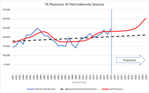
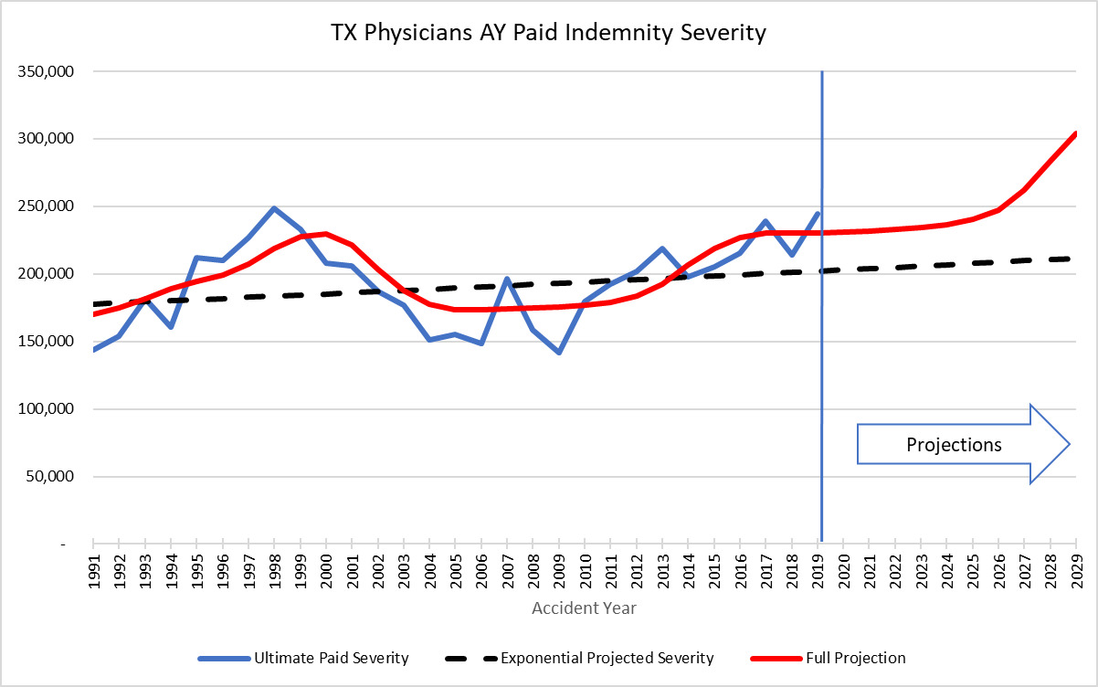
For the going forward model after the tort reform, using an expected 40% level shift jump with 2.5% long term exponential trend, the resulting cyclical trend compares to the developed AY severity trend as follows:

The point here is that it would be extremely difficult to model this pattern using standard regression techniques.

6.2. Frequency Projections of Tort Reform

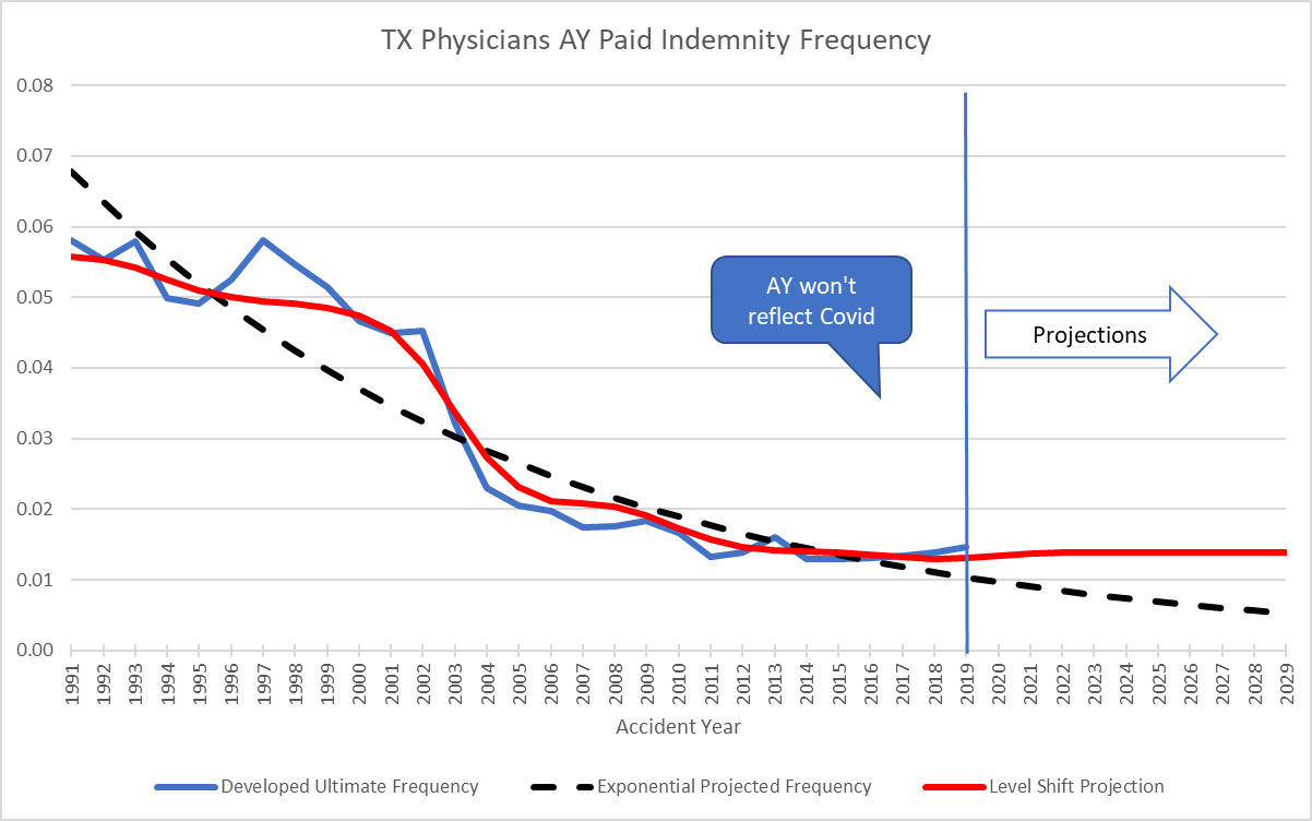
The Level Shift model can also be used to estimate historic frequency trend. This capability comes in handy when there is an external change that affects frequency. Normally, the null hypothesis for MedMal frequency trend is that there is no trend – 0% exponential trend. However, there can be many external things that create a change in frequency such as tort reforms, medical advances, and risk management. A very good example of an external force that affects frequency is the recent COVID pandemic. The pandemic shut down the courts for two years which delayed many payments. The decrease in frequency due to COVID is very evident in the data when you look at it on a CY paid basis.

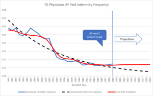
The following graph is a snapshot of the years before and after the tort reform in TX that illustrates the drop in frequency seen when a state initiates a hard cap on pain and suffering. Since the NPDB represents all claims paid against physicians in the state, the state population (total potential patients) would be a reasonable exposure base to use in order to calculate frequency for examining trend. Between 2005 and 2006, the frequency dropped 60%.

So, using a vector of 0% for every year except for -60% in 2005 coupled with an AY claims closing pattern rather than payout pattern, translates into AY trend factors and compares to the AY development method as follows:

When the frequency starts to drop in the standard AY development method, it is difficult to properly project how far it will actually decrease. However, using the CY method, all that is needed is the 60% drop factor to properly work in the subsequent AY or RY trends. When the big drop in frequency is observed on a CY basis in 2005, it can be worked into the trend factors immediately. It is possible to study the effects of the different tort reforms across the different states and come up with a factor that is automatically worked in when tort reform is initiated. Or for the opposite case, if a state removes tort reforms, the adjustment can be made immediately using the CY Level Shift method combined with an estimate as to the percent change one expects due to the tort reform. A benefit of using the Level Shift method is that a jump in severity or change in frequency level is observed much easier and faster than looking at standard RY or AY development triangles.

7. RESULTS AND CONCLUSION

Looking at historical MedMal losses on a calendar year paid/closed basis gives a much clearer picture as to what is happening at different times. These calendar year trends clearly exhibit shifts that are not handled well by fitting exponential curves. At a minimum, whether you believe in a cyclical stair step pattern or not, reviewing the CY paid average severity can be used as an early warning system that some sort of change is going on in the data.

The Level Shift model accounts for these spikes by adding a step function to the projection of future severity trends on a calendar year basis. The size and timing of the steps are analyzed separately for each state based on its own available historic loss data. The idea of adding a step function can be extended to other situations where an infrequent or one-time major external change moves the trend temporarily off course. Adjusting the model is easy by changing the CY vector to reflect any changes.

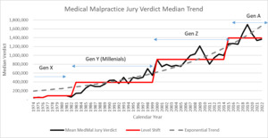
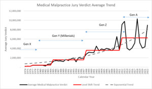
While this methodology represents an improvement to accurately modeling social trend, it also raises some questions. These Level Shifts have now happened at least 4 times in recorded MedMal insurance history. My analysis done in 2010 used this model to successfully project the next CY jump in social inflation that began in 2016 for the MedMal industry. At that time, evidence from the JVR data (Figure 3.2.3) showed that there might have been a jump in average jury verdicts in 2011 which would be an indicator that settlement values would increase. When I have presented this model to various industry personnel, the question I get most often is what causes this cycle of level shifts or social inflation? Using alternative jury verdict data sources (Westlaw) (“Thomson Reuters Westlaw Data Summary,” n.d.), I have used Westlaw’s calculated median and average MedMal jury verdict data to extend the graph subsequent to the JVR data from figure 3.2.3. Please note that this data is on a different basis than the original JVR data and may not be as complete, yet it shows a similar pattern.

So, the jump we saw at the end of the JVR data in Figure 3.2.3 has continued at a higher average level although with much more variation. Here I have mapped the jury verdict step function against commonly used Generational Definitions. An explanation for social inflation in MedMal insurance trends may be the relationship between the changes in the definition of generations and the jumps in jury verdicts. “Generations are one way to group age cohorts. A generation typically refers to groups of people born over a 15–20-year span.” (Pew Research Center 2015)

---

Abbreviations and notations

Biography of Author

Elizabeth Wellington (Betsy) is semi-retired but still doing occasional consulting work. Ms. Wellington provides underwriting and actuarial consulting services to reinsurers and insurance companies specializing in Medical Malpractice. She spent over 20 years working for both reinsurance and primary insurance companies before starting her own consulting operation at the request of industry colleagues. Ms. Wellington has a degree in Business Administration from the University of California at Berkeley and a master’s in arts administration from Indiana University. She is a Fellow of the CAS. She has been a presenter at CARE meetings and CAS meetings on Medical Malpractice topics. She has also been a past member of Exam, University Liaison, and Scholarship committees. She is co-author of "Identifying and Pricing Managed Care Errors and Omissions Exposures " published in the 1997 Call Paper Program. In her free time, Betsy plays piano in a Big Band and Harp and Cello for local events and orchestras and plays competitive Bridge.

Acknowledgments

The author would like to thank her colleagues Kristen Clark, Merle Parrett, Courtney Scott and Dr. John Scheuermann for their input and review of this work.

Contact

xactuary@gmail.com

---

1. A quick note about using the NPDB for severity analysis. There are several states where the Physician severity is so high that average severity is clearly affected by policy limit capping. For example, Connecticut has an average severity approaching $1M, which is the common policy limit held by physicians. Florida has a very small statutory required limit. This is something to be aware of when using the NPDB for analysis.