Machine Learning and Ratemaking: Assessing Performance of Four Popular Algorithms for Modeling Auto Insurance Pure Premium

1. Introduction

Actuaries are tasked with the seemingly impossible role of predicting the future. Actuaries involved with ratemaking are responsible for predicting future claims. Next to using a crystal ball, the best methods for predicting future claims involve complex algorithms that leverage known characteristics of an insured to estimate pure premium. Generalized Linear Models (GLMs) have become standard practice in property & casualty (P&C) pricing. These widely adopted models capture the relationship between a response variable^[1] and explanatory variables or predictors^[2] by transforming a linear combination of predictors and coefficients by a link function (Goldburd et al. 2020). As a natural next step, Fujita et al. (2020) developed the Accurate Generalized Linear Model (AGLM) that builds upon GLMs but is “equipped with recent data science techniques” to achieve “high interpretability^[3] and high predictive accuracy.” Recently, more complex machine learning algorithms have proliferated in the data science industry. With faster execution and predictive performance, it is logical for actuaries to explore the possibility of leveraging these algorithms in ratemaking exercises. Chen and Guestrin took the world by storm in 2016 with the publication of their implementation of eXtreme Gradient Boosting (XGBoost), which improves upon the gradient tree boosting algorithm structure with increased speed and model performance. Neural networks, which transform a series of neurons between input, hidden, and output layers via an activation function, have also gained popularity (Jain 2018).

This paper begins by providing a brief overview of GLM, AGLM, XGBoost, and neural network algorithms. We then discuss the findings related to model development and performance of these algorithms for predicting pure premium on a dataset of French automobile insurance.

2. Model Overview

2.1. GLM: Generalized Linear Model

Generalized linear models (GLMs) are widely used by actuaries for ratemaking in P&C insurance. There is extensive literature on the subject, however Goldburd et al. (2020) released a comprehensive resource related to GLMs for P&C insurance ratemaking. Readers are encouraged to reference GLMs for Insurance Rating^[4] for detailed information about GLMs.

2.2. AGLM: Accurate Generalized Linear Model

In 2020, Fujita, Iwasawa, Kondo, and Tanaka outlined the Accurate Generalized Linear Model (AGLM), which is “based on GLM and equipped with recent data science techniques.” Fujita et al. (2020) highlight that a large concern in predictive modeling is the lack of interpretability of complex machine learning (ML) and artificial intelligence (AI) models. Thus, in GLM-like fashion, the team maintained a one-to-one relationship between predictors and the response for a clearer illustration of how explanatory variables contribute to the response. Fujita et al. (2020) also developed AGLM to achieve high predictive accuracy through discretization of numerical features, coding of numerical features with dummy variables, and regularization.

2.3. XGBoost: eXtreme Gradient Boosting

In 2016, Chen and Guestrin published an article about eXtreme Gradient Boosting (XGBoost) which leverages existing gradient tree boosting techniques to create a faster, highly scalable, and better performing machine learning algorithm. Labram (2019) does an excellent job of explaining how the XGBoost algorithm works at a high level in an article published for the Institute and Faculty of Actuaries in the UK. They highlight how the Gradient Boosting algorithm is a boosted decision tree that sequentially improves the model by targeting reduced residual prediction errors in each tree when compared to the last. XGBoost is an extension of this methodology with optimizations including parallelization of certain processes for increased speed, better sparse data handling, faster searches for splitting points, and improved identification of stopping points for tree growth.

2.4. Neural networks

The R package used for investigation of neural networks in this paper is based on a “feedforward artificial neural network” (Deep Learning (Neural Networks) — H2O 3.38.0.2 documentation^[5]) often referred to as an ANN or deep neural network (DNN). Feedforward ANNs are comprised of an input layer, which corresponds to the model features, one or more hidden layers, and an output layer (Jain 2018). Each layer consists of neurons, which Candel and LeDell (2022) describe as the basic unit of an ANN. Neurons between layers are interconnected and transmit data through the model. In the case of regression, the output layer will consist of a single neuron.

3. Model Performance and Considerations

To compare the performance of GLM, AGLM, XGBoost, and neural networks in predicting pure premium, we sought to develop a framework for tuning models and evaluating performance on a test dataset. We utilized R and the Tidymodels framework^[6] to create a series of scripts to pre-process data, split data through cross-validation, tune models, and export evaluation metrics for analysis and comparison. We utilized 5-fold cross-validation for our research where 80% of the data was used for training and 20% was used for testing of the models in each fold.

3.1. Data source

We utilized the freMTPL2freq and freMTPL2sev datasets from the CASdatasets package in R (Dutang and Charpentier 2020). These datasets include policy numbers, risk features, and claim amounts for 677,991 observations from French motor third-party liability insurance. The response variable for our research is ClaimAmount. Please refer to Appendix A for a list of variables used from both datasets.

We leveraged existing R packages to tune our models. The packages as well as notes on parameter selections are included in Appendix B.

3.2. Does an optimal model exist?

To evaluate model performance, we used 5-fold cross-validation and produced the following quantitative evaluation metrics:

1. Mean Absolute Error (MAE)

2. Root Mean Squared Error (RMSE)

3. 90th Quantile Absolute Error (90 QAE)

4. 95th Quantile Absolute Error (95 QAE)

5. Root Mean Square Log Error (RMSLE)

6. Mean Absolute Percentage Error (MAPE)

7. 90th Quantile Absolute Percentage Error (90 QAPE)

The average results for each algorithm, incorporating cross-validation, are included in Table 1.

Based on the metrics in Table 1, we could be tempted to conclude that neural networks are the optimal choice for predicting future claim amounts. In fact, in one of the cross-validation folds, the neural network has the lowest metrics for all models in all folds.

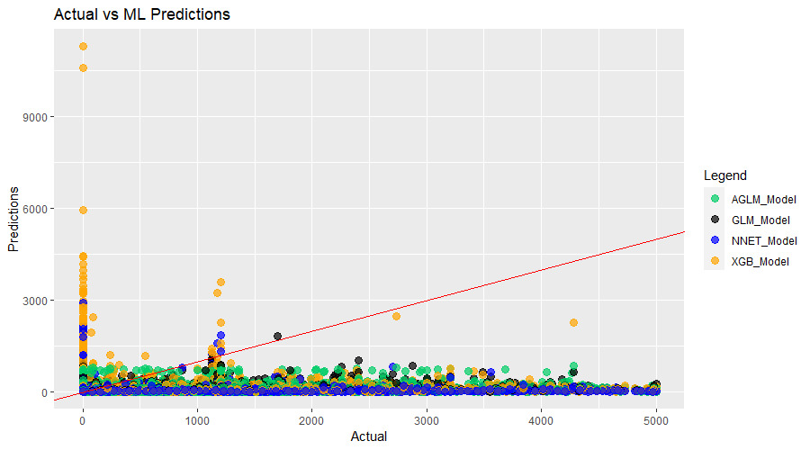
Included below in Figure 1 is a scatterplot of predicted claim amounts against actual claim amounts for each algorithm for that fold. If instead the plot is used as the primary evaluation criteria, it is unlikely that the neural network would be selected as the optimal model. In this fold it is consistently underpredicting pure premium. Theoretically you can understand how an over-trained neural network could achieve this outcome, since the total frequency of TPL claims in this dataset is approximately 7.4%.

Figure 1.Plot of actual claim amounts vs predictions

Corresponds to results from a single cross-validation fold. y = x line included in red for reference. Only observations corresponding to claims less than $5,000 are included.

Conversely, another cross-validation fold has comparatively worse quantitative metrics. Figure 2 corresponds to that fold. Even though the evaluation metrics are worse than the fold described above, the neural network’s predictions appear to be more reasonable qualitatively, following closer patterns to the other models.

Figure 2.Plot of actual claim amounts vs predictions

Corresponds to results from a single cross-validation fold. Line y = x included in red for reference. Only observations corresponding to claims less than $5,000 are included.

Through this exercise, we struggled with whether we could categorize one of models developed as the optimal model. The brief example above illustrates the subjective nature of such a question. Hence, we thought it would be more fitting to discuss the models on a comparative basis according to their quantitative and qualitative performances as well as overall pros and cons.

3.3. GLM discussion

GLMs have been an actuarial pricing standard for many decades. Unsurprisingly, there are many positives associated with GLMs. Firstly, since GLMs are so widely adopted in the actuarial community, there is an extensive array of literature available to support model development processes. Many experienced pricing actuaries will already be familiar with GLMs. Due to the abundance of resources, learning curves will likely be much flatter for new or experienced actuaries when implementing or optimizing a new GLM model. Secondly, model output from a GLM is quite simple to implement in most common rating engines. Lastly, GLMs have a high level of interpretability which makes it much easier to explain the relationship between predictors and output. This is extremely useful for actuaries who will often be tasked to explain pricing models to non-actuarial stakeholders, including regulators.

Though GLMs have many advantages, they are not perfect. Fujita et al. (2020) highlight that there is “trade-off between high interpretability and high prediction accuracy.” Based on the quantitative and qualitative metrics in section 3.2, GLMs had worse overall predictive accuracy compared to more complex models like XGBoost and neural networks. In an increasingly competitive insurance market where customers have access to a wide range of quotes, it is essential for actuaries to price policies as accurately as possible. At the expense of interpretability, pricing actuaries may consider moving towards other models such as those described below.

3.4. AGLM discussion

Fujita et al. (2020) developed AGLM with the goal of balancing the interpretability of GLMs with the improved predictive accuracy of newer data science techniques. They conducted a numerical experiment using AGLM to predict frequency that showed that AGLM was more predictively accurate than a GLM, General Additive Model (GAM), and Gradient Boosting Machine (GBM). Through our research, we struggled with developing an AGLM model for pure premium directly. We also encountered other logistical constraints, such as negative predictions and had to manually set the floor as 0 for predictions produced under AGLM. In our research, AGLM generally had worse quantitative and qualitative performance metrics when compared to all other pure premium models, including GLM.

We believe that a limitation in the R aglm package could be one of the factors contributing to the underperformance of our AGLM model compared to the experiment described by Fujita et al. (2020). The aglm^[7] package in R only supports gaussian, binomial, and Poisson error distributions. In P&C pricing practices, pure premium, frequency, and severity are often assumed to follow Tweedie, Poisson, and gamma error distributions, respectively. We tentatively assumed a gaussian error distribution when developing our AGLM model. Actuaries seeking to leverage the aglm package in R will be required to build separate frequency and severity models, which we did not personally undertake in our research.

3.5. XGBoost discussion

The main appeal of newer machine learning algorithms like XGBoost is high predictive accuracy. XGBoost delivered low quantitative evaluation metrics and strong qualitative performance on most of the models we tuned. XGBoost achieved consistently better quantitative metrics than GLM and AGLM, only beat by a neural network on occasion. However, in those instances when neural networks appeared best, the XGBoost predictions were much more qualitatively reasonable than the neural network. This phenomenon will be discussed further in section 3.6. Compared to our distributional limitations under AGLM, the R package we used allowed us to manually set a Tweedie distribution when developing our XGBoost models.

Despite its high quantitative predictive accuracy, there are concerns that actuaries should take into account when considering XGBoost for predicting pure premiums. XGBoost quickly demonstrates the trade-off between predictive accuracy and interpretability / explainability. Variable importance plots can be utilized to illustrate which predictors contribute more strongly to the response. These are not as straightforward as the direct and quantifiable interpretations that can be drawn from regression coefficients in GLMs. It is also more difficult to explain how XGBoost works to a stakeholder with a non-technical background.

Additionally, XGBoost is sensitive to hyperparameter tuning. We leveraged automated tuning functions in R but found that hyperparameter tuning is computationally intensive with runtimes ranging from one to two days. After tuning, model performance is volatile with evaluation metrics and hyperparameter selections varying widely between folds. We were forced to examine the models produced in each fold and manually select the hyperparameters with the most reasonable results. When investigating each fold, we found that XGBoost models were susceptible to overfitting. Models that achieved very low quantitative performance metrics produced predictions in a small range around $0, which is the most common actual claim amount in the data. This type of performance is less applicable to the context of insurance pricing where premiums must be greater than 0. Hence, hyperparameters from those models would not be appropriate for the purposes of this research.

This process is best understood with a visual example. Table 2 shows the quantitative evaluation metrics for the XGBoost model developed with automated tuning procedures for each cross-validation fold.

Figure 3 corresponds to fold 2, which has the best quantitative metrics. Figure 4 corresponds to fold 3, which has the worst quantitative metrics overall with significant deterioration compared to fold 2. Figure 3 clearly illustrates that some form of overfitting has occurred as all the predictions are in a band near $0. On the other hand, there is more variability in the predictions in Figure 4. In the context of insurance pricing, the model in fold 3 is a more reasonable choice and we would be more likely to extract its hyperparameters for future model development.

Figure 3.Plot of actual claim amounts vs predictions

Corresponds to results from a single cross-validation fold. y = x line included in red for reference

Figure 4.Plot of actual claim amounts vs predictions

Corresponds to results from a single cross-validation fold. y = x line included in red for reference

3.6. Neural network discussion

Neural networks are explored as a modelling alternative for insurance pricing due to expectations of high predictive accuracy. Neural networks produced the lowest quantitative evaluation metrics most of the time with significant improvement compared to GLMs. The R package we leveraged for development of neural networks, H2O, supports a Tweedie error distribution. In addition, we found H2O’s Deep Learning functionality to have an extremely fast runtime compared to AGLM and XGBoost. This allows for easy and quick model tuning and testing. However, not all packages are made equal. We initially tried using the brulee package to develop our neural networks, but found our progress delayed by its long run times. This highlights the importance of investigating and tailoring package and function choices for actuarial exercises, which often require big data.

Similar to XGBoost, a neural network is a black-box algorithm with low interpretability compared to GLMs. Hyperparameters are unintuitive, making selections difficult. It is not straightforward to derive how many epochs, layers, and neurons should be involved based on model context. This limitation should be considered in an insurance pricing context when explainability is an asset for stakeholder communication. Also, like XGBoost, our research found that neural networks were susceptible to overfitting where most predictions were close to $0. But, unlike XGBoost, even when predictions appeared to be more reasonable, actual vs. predicted plots reveal underperformance compared to the other models. For example, Table 3 illustrates the quantitative evaluation metrics for each fold of a neural network we developed. Folds 2 and 3 have the best and worst metrics, respectively.

Figures 3 and 4 above in section 3.5 correspond to folds 2 and 3 in Table 3. Figure 2 clearly demonstrates that slight overfitting was present and caused the strong quantitative metrics. In Figure 3, even though we see that there are comparatively larger predictions, the other models’ predictions appear much more reasonable. We encountered this phenomenon through most of our testing and have seen that neural networks have struggled to predict large claims well.

3.7. Other evaluation metrics

3.7.1. Decile charts

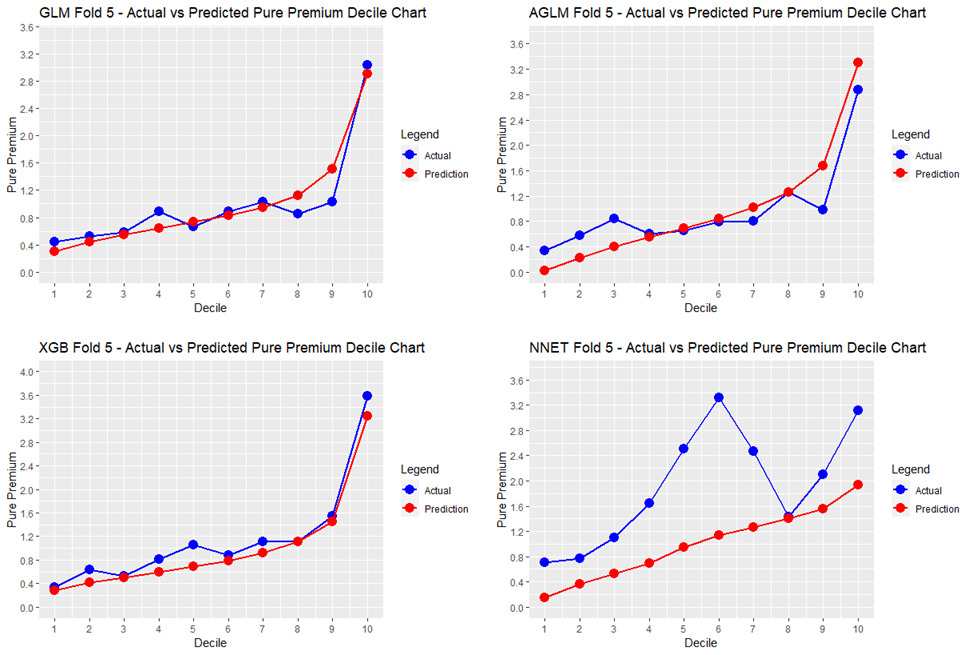
Goldburd et al. (2020) outline a procedure for pricing actuaries to develop quantile plots^[8], which illustrate how well a model identifies the best and worst risks. The procedure involves sorting data points based on the predicted pure premium and plotting the average predicted pure premium and average actual loss for each quantile, or decile, which we have chosen for our analysis. All data points are divided by the average predicted pure premium to improve interpretability of the result.

Goldburd et al. (2020) highlight three criteria to consider when comparing decile charts. First, we look for monotonicity; good models will cause the quantiles of actual losses to increase with small or few reversals. We examine this qualitatively and can notice that most models have a few small reversals, except for the neural network displaying an unfavorable peak between the 4th and 7th deciles. We also notice that the GLM has a noticeable dip at the 8th and 9th deciles where the XGBoost does not. Secondly, we look at the vertical distance between the first and last quantiles of actual losses; the larger the distance, the better a model is at identifying the best and worst risks. Lastly, we assess predictive accuracy; the actual and predicted pure premium quantiles will align much more closely for a predictively accurate model. The last two criteria can be presented quantitatively, which we have done in Table 4. We have chosen to measure predictive accuracy as the sum of absolute differences between the actual and predicted quantiles.

Based on the charts alone, we can assess that GLM and XGBoost have the fewest and smallest reversals and the lines appear quite close. Table 4 displays that XGBoost has the greatest vertical distance between first and last quantiles of actual losses. This means that XGBoost was best able to distinguish the best and worst risks. The spread between the first and last deciles of actual losses for XGBoost is 0.34 to 3.59. Since we divided all data points by the average predicted pure premium, we can interpret XGBoost’s graph to indicate that the best risks are 66% better than average and the worst risks are 359% worse than average. Table 4 also shows that GLM has the smallest sum of absolute differences between quantiles, with XGBoost being slightly worse. We could conclude that both GLM and XGBoost are the most predictively accurate when using decile charts as a primary evaluation metric.

Figure 5.Decile charts for all models

Corresponds to results from a single cross-validation fold.

3.7.2. Actuarial Lorenz curve and Gini coefficient

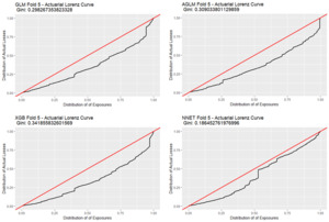
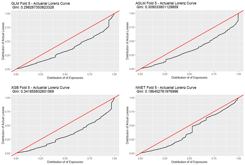
Goldburd et al. (2020) outline a procedure to calculate a Lorenz curve^[9] and corresponding Gini coefficient of an insurance rating plan that can “quantify the ability of the rating plan to differentiate the best and worst risks.” We refer to this as the “Actuarial Lorenz Curve” in our research. These Lorenz curves plot the cumulative distribution of actual losses against the cumulative distribution of exposures after sorting data based on predicted pure premium.

Figure 6 displays the Lorenz curves and Gini coefficients for our models under this methodology. We can interpret the GLM Lorenz curve to indicate that the first 50% of exposures contribute only about 31% of losses. Hence, the model has classified risks well as this means that the worst 50% of exposures contribute a larger proportion, 69%, of losses than the best 50%.

Figure 6.“Actuarial” Lorenz Curves

Corresponds to results from a single cross-validation fold.

4. Conclusion

The goal of this research is to expand the literature available for machine learning applications in actuarial pricing practices through a numerical experiment. It provides a detailed comparison of four different algorithms that can be used to predict pure premium. We examine a variety of quantitative and qualitative evaluation metrics. These assessments draw attention to the importance of using an array of evaluation metrics to determine optimal models.

Our research showed that GLMs continue to be a valuable algorithm for pricing actuaries, while XGBoost, if built correctly, can lead to higher predictive power. Regardless of algorithm that is being employed by an actuary, it is key that a model produces reasonable predictions in addition to having favorable quantitative performance metrics. Actuaries should also be aware of the trade-off between predictive accuracy and interpretability when implementing machine learning models.

4.1. Further research

The topic of machine learning applications for actuarial practices is relatively new and this research cannot encompass all possibilities for the actuarial industry. More research and widespread resources will be crucial to the adoption of machine learning by actuaries. Firstly, we believe it would be valuable to perform a similar exercise on personal auto coverages beyond third-party liability in France, which was used for this experiment. Secondly, machine learning algorithms need not be limited to response prediction. It would be interesting to investigate the use of machine learning algorithms for different purposes such as variable selection from a large list of predictors or creation of new variables. Lastly, we struggled with hyperparameter tuning as there are no unified “best practices” for actuarial models. Actual implementation of machine learning models would benefit from further refinement of hyperparameters and investigation into possible standard selections for different algorithms and response types (e.g., pure premium, frequency, severity).