1. Introduction
McNulty (2021) introduced the concept of Pareto-Gamma mixture in a reinsurance application setting, and provided an overview on the distribution where the Pareto shape parameter follows a Gamma distribution. Motivated by McNulty (2021), this paper focuses on properties of excess severity functions associated with the mixture.
As pointed out in Bahnemann (2015), behaviors of excess severity functions are important characteristics of distributions. How would the excess severity function behave for the mixture proposed in McNulty (2021)? Is it increasing, linear, constant, decreasing or non of the above?
Since Gamma distribution can be viewed as the sum of Exponential distributions (Bahnemann 2015), and so this paper starts with Pareto-Exponential mixture with purpose of revealing clues of meaningful mathematical patterns.
Based on proofs, excess severity function of Pareto-Exponential mixture is increasing and concave (which is neither linear as that of Pareto nor constant as that of Exponential distribution), and for Pareto-Gamma mixture, the excess severity function is increasing with convexity depending on Gamma parameter setting (which is neither decreasing nor convex as Gamma).
Based on insights gained from the above work, numerical computations are conducted for truncated and censored mixtures to illustrate the findings.
2. Pareto-Exponential Mixture
In McNulty (2021), cumulative distribution function (CDF) was deduced first for Pareto-Gamma, based on a combination of results, and then probability density function (PDF) was derived based on CDF.
Here let’s start with derivation of PDF for Pareto-Exponential first.
2.1. Pareto-Exponential Mixture PDF
Suppose the Pareto shape parameter follows an Exponential distribution. Let consider PDF of the mixture:
f(x)=∫∞0fX(x|θ)fθ(θ)dθ=∫∞0θβθ(x+β)(1+θ)⋅λe−λθdθ=λx+β⋅∫∞0θe−(λ+lnx+ββ)θdθ,Letu=(λ+lnx+ββ)θ=λx+β⋅∫∞0ue−udu⋅1(λ+lnx+ββ)2=λ(x+β)(λ+ln(x/β+1))2
2.2. Pareto-Exponential Mixture CDF
Next, let’s look at the CDF There are certain properties must follow to be considered as a cumulative distribution function.
Consider the integral Notice that
∫∞0f(x)dx=∫∞0λ(x+β)(λ+ln(x/β+1))2dx=λ∫∞1d(lnu)(λ+lnu)2,Letu=x/β+1=−λλ+ln(u)|∞1=1
Consider a strictly positive then
S(L)=Pr(X≥L)=∫∞Lf(x)dx=λλ+ln(L/β+1)
and
F(L)=1−S(L)=1−λλ+ln(L/β+1)
2.3. Expectations
Not all expectation values are finite. In terms of this mixture, we look at the integral:
E(x)=∫∞0λx(x+β)(λ+ln(x/β+β))2dx∝∫∞1u−1u⋅1(λ+lnu)2dx,Let u=(x+β)/β>∫21u−1u⋅1(λ+lnu)2du+∫∞2u−u/2u⋅1(λ+lnu)2du⏟∝ finite term+∫∞2eλdw(lnw)2,wherew=ueλ
This expression reconciles with that of McNulty (2021), which does not converge. However, the infinity of expectation should not be a problem as an upper limit could be assigned.
2.4. Excess Severity of Pareto-Exponential Mixture
Per notations defined in Bahnemann (2015), excess severity of a random variable X is defined as which is also called the mean excess claim size at
Proposition 2.1. Excess severity function of the Pareto-Exponential Mixture is increasing and concave.
Proof. Consider
e(x)=∫∞xtf(t)dt−xS(x)S(x)
Let
D(x)=∫∞xtf(t)dt−xS(x)
note that
D′(x)=−xf(x)−S(x)−xS′(x)=−S(x)
we have
e′(x)=−1+f(x)D(x)S2(x)=−1+D(x)λ(x+β)
since for every finite is finite while does not converge, and so
then consider
e″(x)=D′(x)λ(x+β)−λD(x)λ2(x+β)2=−1⋅(S(x))λβ+λ(∫∞xtf(t)dt)λ2(x+β)2⏟
note that the term inside the bracket is positive, thus ◻
2.5. Excess Severity of Truncated and Censored Pareto-Exponential Mixture
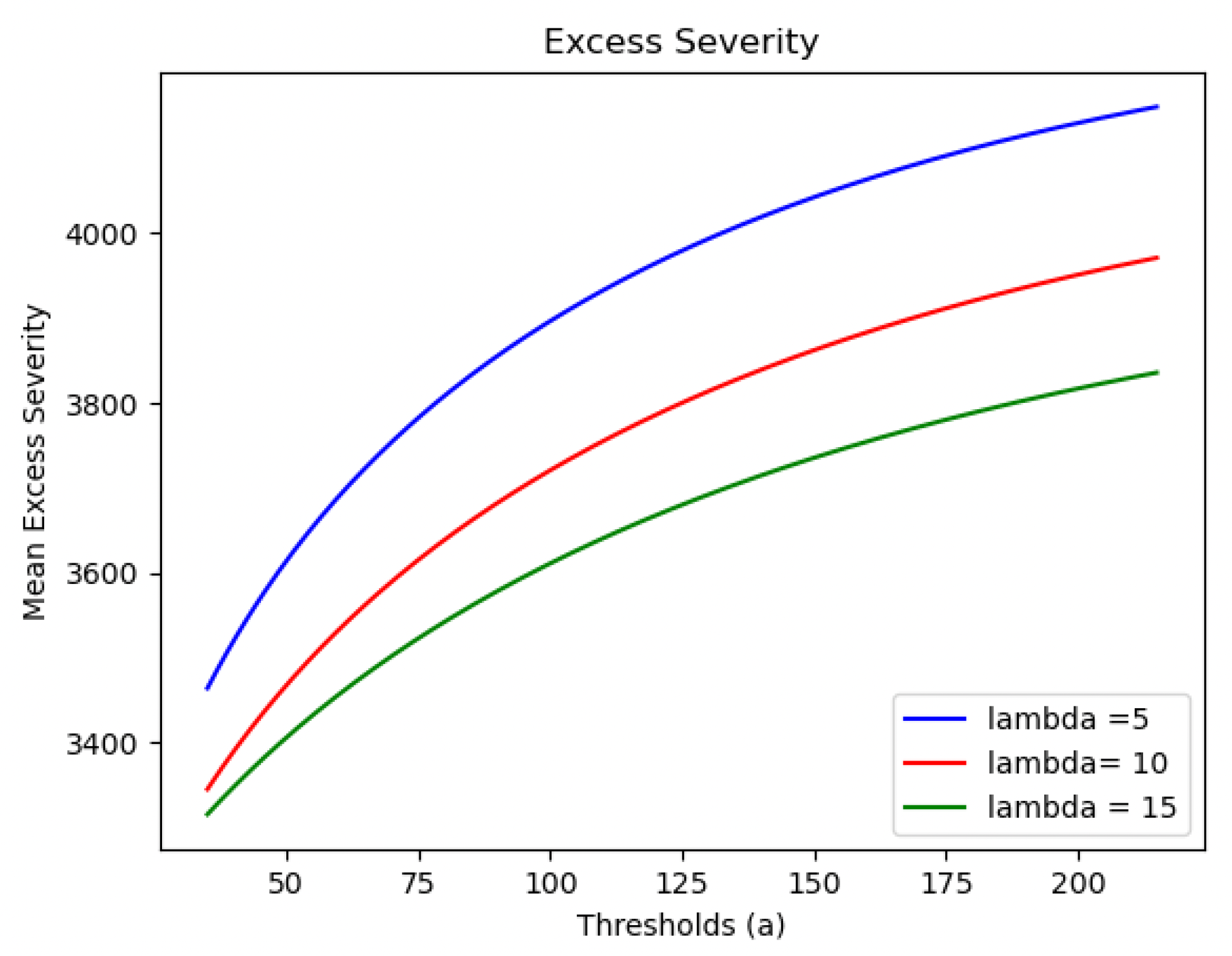
Consider the Pareto-Exponential mixture defined on the domain between and i.e., a truncated and censored Pareto-Exponential distribution. Here can be viewed as the threshold selected, and can be viewed as the maximum possible claim size, or just a large finite number which is significantly above all historical claim sizes.
Let’s look at the excess severity function, and observe how the excess severity varies as the chosen threshold changes.
The theoretical excess severity function of takes the form:
eX(a)=∫Maxf(x)dx+(MS(M)−aS(a))1−F(a)
Consider when . Consider scenarios where M is sufficiently larger than a. Since there is no closed form for the excess severity expression in this case, and so here numerical methods are employed to compute the integral in (1), and to explore excess severity behaviors.
Let and then the plot is as follows:

Caveat
Note that here the condition is sufficiently larger than a) cannot be dropped due to the finite censored point as Otherwise, the increasing property may not hold. Let and so then we have
e′X(a)=−1+I+Qλ⋅(a+β)
Namely, the maximum point needs to satisfy
3. Pareto-Gamma Mixture
Note that there is a slight notation difference between McNulty (2021) and this paper. Here corresponds to in McNulty (2021), and corresponds to in McNulty (2021), and McNulty (2021) assumes the location parameter is fixed and does not include it explicitly in formula, i.e., here corresponds to in McNulty (2021).
The survival fucntion takes the form of
S(x)=λα(λ+ln(x/β+1))α
which is exactly the survival function of Pareto-Exponential mixture raised to
The PDF
f(x)=αS(x)1+1/αλ(x+β)
3.1. Excess Severity of Pareto-Gamma Mixture
Proposition 2. The excess severity function is increasing.
Note that
e(x)=∫∞xtf(t)dt−xS(x)S(x)=D(x)S(x)
e′(x)=−1+f(x)D(x)S2(x)=−1+αS(x)−1+1/αD(x)λ(x+β)>0
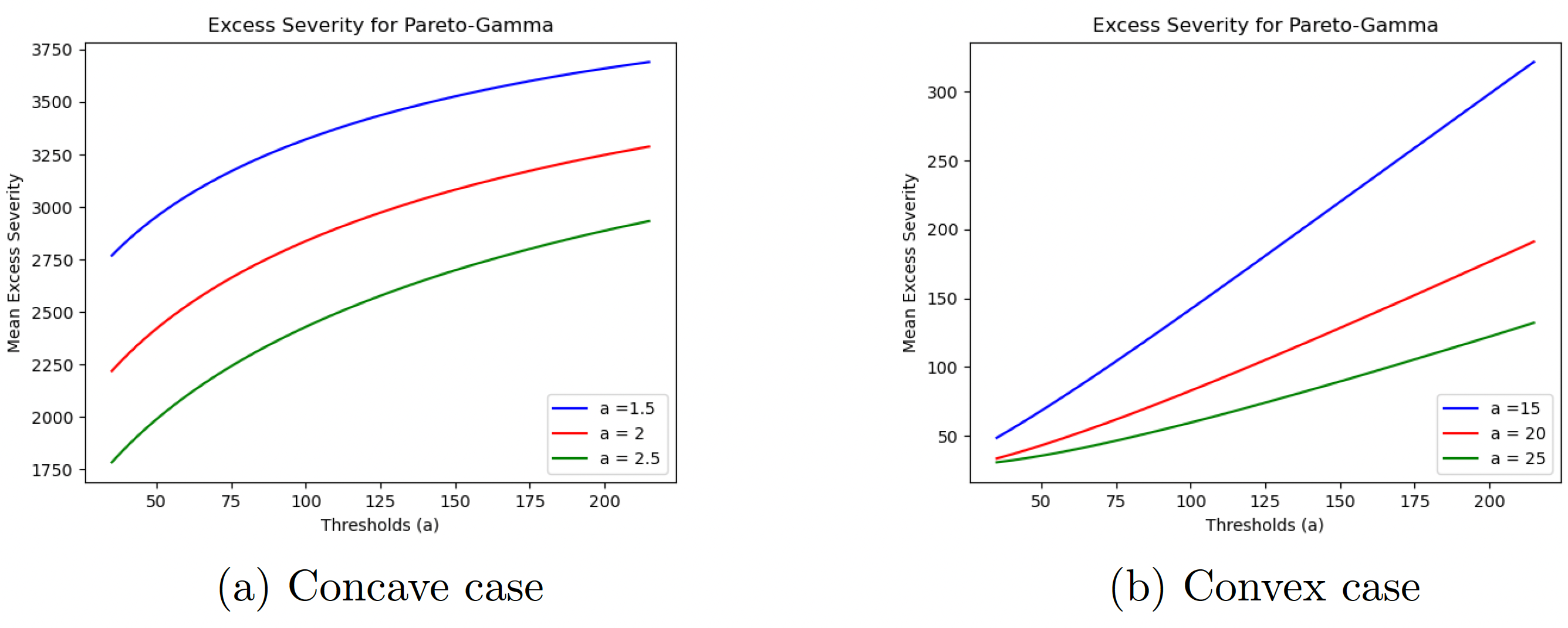
Comments on Convexity[1]
However, the convexity of the excess severity function is not fixed for all values. As increases, the excess severity gradually changes from concave to convex.
3.2. Excess Severity of Truncated and Censored Distributions
Similar to the Pareto-Exponential Mixture, let’s compute the integral in (1) via numerical methods for the Pareto-Gamma mixture and to explore excess severity behaviors. Let and then we have the plot as follows.

Caveat
Note that here the condition is sufficiently larger than a) cannot be dropped due to the finite censored point as Otherwise, the increasing property may not hold.
4. Conclusion
Excess severity functions are indicative of a particular family of distributions. In this paper, excess severity functions of Pareto-Exponential and Pareto-Gamma mixtures are examined. Hopefully, the above results could help further practical modeling.
Note that e″(x)=−1⋅λ(1−α)f(x)S(x)−2−1/αD(x)(x+β)+λα(βS(x)1/α+S(x)−1/α−1∫∞xtf(t)dtλ2(x+β)2For instance, consider when then