Quantifying Reserve Risk Based on Volatility in Triangles of Estimated Ultimate Losses

1. INTRODUCTION

This paper measures the risk from the volatility in a triangle of estimated ultimate losses rather than deriving metrics of risk from the volatility in the underlying paid or incurred triangles. Take a hypothetical omniscient actuary using the perfect crystal ball method. The resulting triangle of estimated ultimate losses would be constant along each accident year row. The development factors on the ultimate losses at each age would be 1. However, in the real world, the resulting estimates will change at each evaluation and the ultimate development factors will be different from 1. Intuitively, the degree of variation in the ultimate losses can be used to measure reserve volatility.

The correlation among the age-to-age factors could have a significant impact on reserve risk. Although the correlations among the age-to-age paid or incurred development factors tend to be positive, correlations among the age-to-age ultimate development factors can be negative. In the context of reserve risk, this means that when using paid or incurred loss triangles, reserve risk with correlation included is often higher than reserve risk calculated without correlation terms. On the other hand, when based on ultimate loss triangles, reserve risk with correlation terms in the formula can sometimes be larger, and at other times lower, than when the correlation terms are omitted.

This paper will also highlight and diagnose irregularities that can arise from use of the variance-covariance matrix when it is derived from columns of development factors. Typically, each entry in an empirical variance-covariance matrix is based on taking the variance and covariance of vectors of the same size. Such a matrix will be well-behaved and have desirable mathematical properties. However, all bets are off when the vectors are of different sizes. In a loss triangle, there are fewer observations in the more mature development age columns. As will be shown, a nominal variance-covariance matrix based on such triangular structure can exhibit surprising pathologies. Another aspect of the “triangle structure problem” is that the later age development factors are more leveraged, yet more impactful. Hence the resulting risk estimates are inherently more unstable. Tentative solutions will be proposed to these problems based on an approach of filling in the triangle of factors and recalibrating the covariance matrix to offset any bias introduced.

1.1. Research Context

There are several ways to estimate reserve risk using historical loss data. Mack (1993) provided the first example, estimating the total run-off reserve risk using paid or incurred loss triangles. Merz and Wuthrich (2008) extended this methodology to evaluate the one-year reserve risk. Robbin (2012) provided a refinement to the Standard Formula used in Solvency II. Rehman and Klugman (2010) proposed using the triangle of estimated ultimate losses to estimate ultimate reserve risk. They assumed that the development factors, rather than losses, follow a log-normal distribution. Siegenthaler (2019) also used a triangle of estimated ultimate losses to derive both a one-year and a total run-off formula, but he used different assumptions and obtained different resulting formulas than Rehman and Klugman.

1.2. Objectives

This paper will introduce the Feng-Robbin method, which makes several specific algorithmic enhancements in estimating reserve risk.^[1]

The approach starts with the triangle model promulgated by Rehman and Klugman. In this model, age-to-age factors of ultimate losses are assumed to be lognormally distributed. The Rehman and Klugman model will be enhanced and extended in several ways:

• Develop a one-year reserve risk estimate.

• Examine the covariance terms and derive a slightly different formula for the total run-off reserve risk.

• Propose solutions to address the “triangle structure problem” that will eliminate potentially anomalous behaviors when raw variance-covariance matrices are used.

• Propose an estimate of the parameter risk component of reserve risk.

1.3. Outline

The remainder of the paper proceeds as follows. Section 2 starts with a general discussion of reserve risk. Section 3 is devoted to presenting the formulas for one-year and total run-off reserve risk estimates. Section 4 simplifies the formulas using matrix notation. Section 5 demonstrates how the raw variance-covariance matrix can go awry and yield a negative overall variance. It then presents several alternatives for addressing the “triangle structure problem.” Section 6 proposes an estimate for parameter error. Section 7 provides a comparison of the various formula-based methods as well as insights gained from examining the application of the methods to numerical data.

This paper will include simple examples to demonstrate the methodology described in each section. In the more substantial examples in Section 7 and Appendix C, different sets of ultimate triangles will be analyzed using a variety of reserving methods, and different methods will be applied to these ultimate loss triangles to calculate reserve risk standard errors.

2. Reserve Risk

What is reserve risk? In the context of this paper, it is the potential for adverse and favorable deviations between the eventual ultimate losses and the latest estimates of ultimate. The very mature accident years should have very little deviation, while the newer accident years could have sizeable volatility.

There are two main drivers of reserve risk. First is the volatility in the underlying loss development data. Such volatility of the underlying development process in turn translates into volatility in the difference between the eventual ultimate losses and the latest estimates on the diagonal. Second is the volatility that stems from the method used to project the ultimate estimates. While some methods are mathematically more stable than others, this does not necessarily imply they produce more accurate estimates of ultimate more quickly.

This paper will develop formulae for ultimate and for one-year reserve risk. The one-year reserve risk measures the volatility of the estimate of ultimate losses over the next year, whereas the ultimate reserve risk, also referred to as total run-off reserve risk, measures the variability of the estimated ultimate losses until all outstanding contract obligations are fulfilled. In the context of Solvency II, the expected unpaid loss is called the undiscounted best estimate and it is assumed to have no built-in prudential margin.

3. One Year and Ultimate Run-off Standard Errors

The main results will be presented in this section, following a summary of the notation shown in Table 1. The notation is largely consistent with that used by Mack, Merz and Wuthrich, and Siegenthaler,^[2] but differs from that used by Rehman and Klugman.^[3]

In addition, Table 2 has the notation for various lognormal and normal distribution parameters:

The estimators for these parameters will be denoted by an accent character $(\widehat{\ \ })$ on top of the variable. The formula for the estimators will be given in Sections 3.3 and 3.4. Additionally, let ${\sigma_{i,j}}^{2}$ denote the covariance between $ln(g_{i})$ and $ln(g_{j}).$ If $i = j,$ then ${\sigma_{i,i}}^{2} = {\sigma_{i}}^{2}$ is the variance of $ln(g_{i}).$ Even though the covariance terms could be negative, we used ${\sigma_{i,j}}^{2}$ instead of the more common $\sigma_{i,j}$ to simplify the collection of terms within the variance-covariance matrix.

Using the above notation, the main result for the one-year standard deviation for the entire triangle is as follows.

$$\begin{align} {\text{StDev}}\left( \sum_{y = 1}^{Y}U_{y,D - y + 2} \right) &= \sum_{y = 1}^{Y}U_{y,D - y + 1\ }\ \\ &\quad \times \ \sqrt{\left( e^{2\widehat{\alpha} + 2{\widehat{\theta}}^{2}} - e^{2\widehat{\alpha} + {\widehat{\theta}}^{2}} \right)} \end{align} \tag{3.01}$$

where $\widehat{\alpha} ≔ \sum_{y = 1}^{Y}r_{y}{\widehat{\mu}}_{D - y + 1}$ and$\ {\widehat{\theta}}^{2} ≔ \sum_{i = 1}^{Y}{\sum_{j = 1}^{Y}r_{i}r_{j}}{{\widehat{\sigma}}_{D - i + 1,D - j + 1}}^{2}$

The main result for the total run-off standard deviation for the entire triangle is as follows.

$$\begin{align} {\text{StDev}}\left( \sum_{y = 1}^{Y}U_{y,D} \right) &= \sum_{y = 1}^{Y}U_{y,D - y + 1}\ \\ &\quad \times \ \sqrt{\left( e^{2\widehat{\omega} + 2{\widehat{\lambda}}^{2}} - e^{2\widehat{\omega} + {\widehat{\lambda}}^{2}} \right)} \end{align} \tag{3.02}$$

where $\widehat{\omega} ≔ \sum_{d = 1}^{D}R_{d}{\widehat{\mu}}_{d}$ and $\hat{\lambda}^2:=\sum_{i=1}^D \sum_{j=1}^D R_i R_j \hat{\sigma}_{i, j}{ }^2$

3.1. Development Model Setup

The setup of this paper is largely consistent with that used by Rehman and Klugman.

For a given line of business with $Y$ accident years and $D$ development periods, historical estimated ultimate losses are arrayed in the usual triangle format as shown in Table 3.

A frequently used quantity is the sum over the latest diagonal $\sum_{y = 1}^{Y}U_{y,\ D - y + 1},$ which represents the sum of the best available estimate of ultimate over all accident years at the time of evaluation.^[4] Estimates in all future development periods are uncertain.

Throughout this paper, the illustrative triangle of ultimate losses in Table 4 will be used to demonstrate the methodology developed.

3.1.1. Ultimate Loss Development Factors

Consistent with Rehman and Klugman’s, and Siegenthaler’s, definitions, the age-to-age ultimate development factor, or UDF, is defined as

$$\begin{align} g_{y,d} ≔ \ \frac{U_{y,\ d + 1}}{U_{y,\ d}}\tag{3.03} \end{align}$$

Similar to the age-to-age development factors for paid or incurred losses, a triangle of such ultimate development factors shown in Table 5 could be computed using the observed ultimate estimates, as illustrated using the same structure as Table 3.

Define the random variable $g_{d}$ as the age-to-age ultimate development factor applicable for ultimate losses from age $d$ to $d$+1. This makes each $g_{y,\ \ d}$ an observed value for $g_{d}$ for $y \leq D - d.$ As later sections of this paper would demonstrate, if the distribution of $g_{d}$ is known, variance of the ultimate losses in future development periods would follow.

The observed age-to-age ultimate development factors for the illustrative triangle are shown in Table 6. For example, 1.0502 in accident year 1 age 2-3 is calculated as 921÷877.

A related concept is the age-to-ultimate ultimate^[5] development factor, $G_{d},$ defined as the product of all age-to-age development from age $d$ up to maturity age $D.$ That is,

$$\begin{matrix} G_{d} = \prod_{j = d}^{D}g_{j}\tag{3.04} \end{matrix}$$

The estimation of age-to-ultimate UDF is computationally similar to the age-to-ultimate paid or incurred loss development factors and could be used similarly.

3.1.2. Accident Year Weight Factors

To address the different volume of exposure in each accident year, a weight factor $r_{y}$ is calculated for each accident year $y$ as a proportion of the latest estimate of ultimate losses:

$$\begin{matrix} r_{y} = \ \frac{U_{y,D - y + 1}}{\sum_{j = 1}^{Y}U_{j,\ D - j + 1\ }}\tag{3.05} \end{matrix}$$

It is easy to check that $\sum_{y = 1}^{Y}r_{y} = 1.$

For total run-off risks, a cumulative weight is defined for each age as follows:

$$\begin{matrix} R_{d} ≔ \sum_{j = Y - d + 1}^{Y}{r_{j}\ }\tag{3.06} \end{matrix}$$

For the illustrative triangle, the weight factors are shown in Table 7.

3.2. Model Assumptions

Model assumptions are entirely consistent with those used in Rehman and Klugman (2010). The main assumption is that age-to-age UDFs for each development age follow a log-normal distribution for all origin periods. It follows that the logarithm of UDFs follow a normal distribution. No assumption is made regarding the independence of the age-to-age ultimate development factors, and no assumption is required regarding the method of determining the ultimate loss estimates at each calendar year. Mathematically,

$$g_{d}\ \sim\ LogNormal\ (\mu_{d},\ {\sigma_{d}}^{2})$$

The mean, variance and covariance of $g_{d}$ can be initially estimated by taking the logarithm of the triangle of UDFs.^[6]

Following the methodology developed in Rehman and Klugman, $\mu_{d}$ and$\ {\sigma_{d}}^{2}$ could be estimated using the following sample mean and variance formulae.

$$\begin{matrix} {\widehat{\mu}}_{d} ≔ \ \frac{\sum_{y = 1}^{Y - d}{{\text{ln}(g}_{y,d})\ }}{Y - d}\ \tag{3.07} \end{matrix}$$

$$\begin{matrix} {{\widehat{\sigma}}_{d}}^{2} ≔ \ \frac{\sum_{y = 1}^{Y - d}{{{(\text{ln}(g}_{y,d}) - {\widehat{\mu}}_{d})}^{2}\ }}{Y - d - 1}\ \tag{3.08} \end{matrix}$$

The observed logarithms of the age-to-age ultimate development factors for the illustrative triangle are presented in Table 8.

The estimated unadjusted mean and variance of each log UDF factor is shown in Table 9.

The variance-covariance matrix presented in Table 10 is adjusted according to the full-adjustment procedure described in Section 5.2.3. This guarantees a positive calculated variance.

It follows from the definition of $g_{d}$ that

$$\begin{matrix} {\widehat{U}}_{y,\ d + 1} = \ U_{y,\ d}\ \times \ g_{d}\ \tag{3.09} \end{matrix}$$

The above equation implicitly assumes that future ultimate losses can be predicted using past ultimate losses. This relationship would fail to hold if there is extraneous information indicating future changes in reserving methodology, and such future changes are not reflected in the past data triangle of $U_{y,\ d}$'s. In such situations, computed risk amounts must be manually adjusted. Retroactive adjustments of historical ultimate losses could also be made.

3.2.1. Simplifying Assumptions

This paper follows Rehman and Klugman’s use of a first-degree Taylor series approximation for the exponential and logarithmic functions. It is assumed that if $x \approx 0,$ $e^{x} \approx 1 + x;$ if $x \approx 1,$ $\ln(x) \approx x - 1.$ For a triangle of ultimate losses, age-to-age$\ g$ factors are approximately 1, thus $\ln(g)$ is approximately 0. The exponential approximation is used where $x = \ln(g)$ while the logarithmic approximation is used where $x = g.$ Consequently, these approximations are appropriate. These approximations are utilized in the proof in Appendix A.

3.3. Standard Error of Ultimate Run-off Reserve Risk

In this section, a slightly modified version of Rehman and Klugman’s formula is presented due to a more detailed analysis of covariance terms. The result is similar to Rehman (2016).

3.3.1. Total Run-off Reserve Risk – Single Accident Year

The ultimate estimate at maturity for a single accident year is $U_{y,D}.$ It has variance

$$\begin{align} \text{Var}\left\lbrack U_{y,D} \right\rbrack &= {U_{y,D - y + 1}}^{2} \times \ \text{Var}\left\lbrack \frac{U_{y,D}}{U_{y,D - y + 1}} \right\rbrack \\&= {U_{y,D - y + 1}}^{2}\ \times \text{Var}\ \left\lbrack G_{D - y + 1} \right\rbrack \end{align}$$

Here $U_{y,D - y + 1}$ is the latest known ultimate estimate for accident year $y.$ Since $G_{D - y + 1} = \ \prod_{d = D - y + 1}^{D}g_{d}$ is distributed log-normally, $\ln{(G_{D - y + 1}}) = \ \sum_{d = D - y + 1}^{D}{ln(}g_{d})$ is distributed normally with associated mean and variance given by

$$\begin{matrix} {\widehat{\omega}}_{y} ≔ E\left\lbrack \sum_{d = D - y + 1}^{D}{ln(}g_{d}) \right\rbrack = \sum_{d = D - y + 1}^{D}{\widehat{\mu}}_{d}\ \tag{3.10} \end{matrix}$$

$$\begin{align} {{\widehat{\lambda}}_{y}}^{2} &≔ Var\left\lbrack \sum_{d = D - y + 1}^{D}{ln(}g_{d}) \right\rbrack \\ &= \ \sum_{i = D - y + 1}^{D}{\sum_{j = D - y + 1}^{D}{{\widehat{\sigma}}_{i,j}}^{2}} \end{align} \tag{3.11}$$

In the above equations, ${\widehat{\mu}}_{d}$ is the mean of the $\text{ln}(g_{d})$ and ${{\widehat{\sigma}}_{i,j}}^{2}$ is the covariance between $\text{ln}(g_{i})$ and $ln(g_{j}).$ If $i = j,$ ${{\widehat{\sigma}}_{i,i}}^{2} = {{\widehat{\sigma}}_{i}}^{2}$ is the sample variance of $\text{ln}(g_{i}).$

Thus, the standard error of total run-off reserve risk for a single accident year is given by

$$\begin{align} \text{StDev}\left( U_{y,D} \right) &= U_{y,D - y + 1}\ \\ &\quad \times \ \sqrt{\left( e^{2{\widehat{\omega}}_{y} + 2{{\widehat{\lambda}}_{y}}^{2}} - e^{2{\widehat{\omega}}_{y} + {{\widehat{\lambda}}_{y}}^{2}} \right)} \tag{3.12} \end{align}$$

Equations 3.10 through 3.12 produce identical results as the Rehman-Klugman method for a single accident year.

Using the illustrative triangle, the results for each accident year are given in Table 11.

3.3.2. Total Run-off Reserve Risk – All Accident Years Combined

The ultimate estimate at maturity for the sum of all accident year is $\sum_{y = 1}^{Y}U_{y,D}.$ This quantity has variance

$$\begin{align} \operatorname{Var}\left[\sum_{y=1}^Y U_{y, D}\right]&=\left(\sum_{y=1}^Y U_{y, D-y+1}\right)^2 \\ &\quad \times \operatorname{Var}\left[\frac{\sum_{y=1}^Y U_{y, D}}{\sum_{y=1}^Y U_{y, D-y+1}}\right] \end{align}$$

Lemma A.1 in the Appendix demonstrates that

$$\ln\left( \frac{\sum_{y = 1}^{Y}U_{y,\ D}}{\sum_{y = 1}^{Y}U_{y,D - y + 1\ }} \right) \approx \ \sum_{d = 1}^{D}{R_{d}\text{ln}(g_{d})}$$

Since $g_{d}$ has a lognormal distribution, $\ln\left( g_{d} \right)$ is normally distributed with mean ${\widehat{\mu}}_{d}$ and variance ${{\widehat{\sigma}}_{d}}^{2}.$ The linear combination of normally distributed random variables with coefficients $R_{d}$ is a normally distributed random variable with mean and variance given by:

$$\begin{matrix} \widehat{\omega} ≔ E\left\lbrack \ \sum_{d = 1}^{D}R_{d}ln\left( g_{d} \right) \right\rbrack = \sum_{d = 1}^{D}R_{d}{\widehat{\mu}}_{d} \tag{3.13} \end{matrix}$$

$$\begin{matrix} {\widehat{\lambda}}^{2} ≔ Var\left\lbrack \sum_{d = 1}^{D}R_{d}ln\left( g_{d} \right) \right\rbrack = \ \sum_{i = 1}^{D}{\sum_{j = 1}^{D}R_{i}R_{j}}{{\widehat{\sigma}}_{i,j}}^{2} \tag{3.14} \end{matrix}$$

Note that $\widehat{\omega}$ and ${\widehat{\lambda}}^{2}$ are total run-off estimators for the entire triangle, whereas ${\widehat{\mu}}_{d}$ and ${{\widehat{\sigma}}_{i,j}}^{2}$ are estimators for specific ages. It is also important to distinguish ${\widehat{\omega}}_{y}$ from $\widehat{\omega}$ and ${\widehat{\lambda}}_{y}$ from ${\widehat{\lambda}}^{2}.$

In some cases, the formula for ${\widehat{\lambda}}^{2}$ above yields an anomalous negative variance if the raw variance-covariance matrix is used. This issue is further explored in Section 5. Starting from Equation 3.14, the Feng-Robbin method diverges from the Rehman-Klugman method.

Recovering the variance of the lognormal distribution yields

$$\text{Var}\left( \frac{\sum_{y = 1}^{Y}U_{y,\ D}}{\sum_{y = 1}^{Y}U_{y,D - y + 1\ }} \right) = e^{2\widehat{\omega} + 2{\widehat{\lambda}}^{2}} - e^{2\widehat{\omega} + {\widehat{\lambda}}^{2}}$$

The completed formula for the standard error of total run-off reserve risk is

$$\begin{align} \text{StDev}\left( \sum_{y = 1}^{Y}U_{y,D} \right) &= \sum_{y = 1}^{Y}U_{y,D - y + 1}\ \\ &\quad \times \ \sqrt{\left( e^{2\widehat{\omega} + 2{\widehat{\lambda}}^{2}} - e^{2\widehat{\omega} + {\widehat{\lambda}}^{2}} \right)}\tag{3.15} \end{align}$$

Using the illustrative triangle, the total run-off results for the sum of all accident years is given in Table 12.

3.4. Standard Error of One-Year Reserve Risk

This is a new result not covered by either Rehman and Klugman (2010) or Rehman (2016).

3.4.1. One-year Reserve Risk – Single Accident Year

The ultimate estimate for a single accident year evaluated 12 months in the future is $U_{y,D - y + 2}.$ The variance of this quantity is

$$\begin{align} \text{Var}\left\lbrack U_{y,D - y + 2} \right\rbrack &= {U_{y,D - y + 1}}^{2} \times \ \text{Var}\left\lbrack \frac{U_{y,D - y + 2}}{U_{y,D - y + 1}} \right\rbrack \\ &= {U_{y,D - y + 1}}^{2}\ \times \text{Var}\ \left\lbrack g_{D - y + 1} \right\rbrack \end{align}$$

Here $U_{y,D - y + 1}$ is the latest known ultimate estimate for accident year $y.$ Random variable $g_{D - y + 1}$ has a lognormal distribution with associated mean and variance parameters given by

$$\begin{matrix} {\widehat{\alpha}}_{y} ≔ \text{E}\left\lbrack \ln{(g_{D - y + 1})} \right\rbrack = {\widehat{\mu}}_{D - y + 1}\tag{3.16} \end{matrix}$$

$$\begin{matrix} {{\widehat{\theta}}_{y}}^{2} ≔ \text{Var}\left\lbrack \ln{(g_{D - y + 1})} \right\rbrack = \ {{\widehat{\sigma}}_{D - y + 1}}^{2}\tag{3.17} \end{matrix}$$

Thus, the standard error of one-year reserve risk for a single accident year is given by

$$\begin{align} \text{StDev}\left( U_{y,D - y + 2} \right) &= U_{y,D - y + 1}\ \\ &\quad \times \ \sqrt{\left( e^{2{\widehat{\alpha}}_{y} + 2{{\widehat{\theta}}_{y}}^{2}} - e^{2{\widehat{\alpha}}_{y} + {{\widehat{\theta}}_{y}}^{2}} \right)}\tag{3.18} \end{align}$$

Using the illustrative triangle, the one-year results for each accident year are given in Table 13.

3.4.2. One-year Reserve Risk – All Accident Years Combined

The ultimate estimate for the sum of all accident years evaluated 12 months in the future is $\sum_{y = 1}^{Y}U_{y,D - y + 2}.$ The variance of this quantity is expressed as

$$\begin{align} \operatorname{Var}\left[\sum_{y=1}^Y U_{y, D-y+2}\right]&=\left(\sum_{y=1}^Y U_{y, D-y+1}\right)^2 \\ &\quad \times \operatorname{Var}\left[\frac{\sum_{y=1}^Y U_{y, D-y+2}}{\sum_{y=1}^Y U_{y, D-y+1}}\right] \end{align}$$

Lemma A.2 in the Appendix demonstrates that

$$\ln\left( \frac{\sum_{y = 1}^{Y}U_{y,D - y + 2}}{\sum_{y = 1}^{Y}U_{y,D - y + 1\ }} \right) \approx \ \sum_{y = 1}^{Y}r_{y}\ln\left( g_{D - y + 1} \right)$$

Since $g_{D - y + 1}$ has a lognormal distribution, $\ln\left( g_{D - y + 1} \right)$ has a normal distribution with mean ${\widehat{\mu}}_{D - y + 1}$ and variance ${{\widehat{\sigma}}_{D - y + 1}}^{2}.$ The linear combination of such normal distributions with coefficients $r_{y}$ is another normal distribution with mean and variance given as follows:

$$\begin{matrix} \widehat{\alpha} ≔ \text{E}\left\lbrack \ \sum_{y = 1}^{Y}r_{y}\ln\left( g_{D - y + 1} \right) \right\rbrack = \sum_{y = 1}^{Y}r_{y}{\widehat{\mu}}_{D - y + 1}\tag{3.19} \end{matrix}$$

$$\begin{align} {\widehat{\theta}}^{2} &≔ \text{Var}\left\lbrack \sum_{y = 1}^{Y}r_{y}\ln\left( g_{D - y + 1} \right) \right\rbrack \\ &= \ \sum_{i = 1}^{Y}{\sum_{j = 1}^{Y}r_{i}r_{j}}{{\widehat{\sigma}}_{D - i + 1,D - j + 1}}^{2}\tag{3.20} \end{align}$$

Note that $\widehat{\alpha}$ and ${\widehat{\theta}}^{2}$ are estimators for the entire triangle, whereas ${\widehat{\mu}}_{d}$ and ${{\widehat{\sigma}}_{i,j}}^{2}$ are estimators for specific ages. Additionally, ${{\widehat{\sigma}}_{D - i + 1,D - j + 1}}^{2}$ is a covariance term between development age $i$ and $j$ when $i \neq j.$ It is also important to distinguish $\widehat{\alpha}$ and ${\widehat{\theta}}^{2}$ from ${\widehat{\alpha}}_{y}$ and ${\widehat{\theta}}_{y},$ and from $\widehat{\omega}$ and ${\widehat{\lambda}}^{2}$ used for the total run-off reserve risk.

Recovering the variance of the lognormal distribution yields

$$\text{Var}\left( \frac{\sum_{y = 1}^{Y}U_{y,D - y + 2}}{\sum_{y = 1}^{Y}U_{y,D - y + 1\ }} \right) = e^{2\widehat{\alpha} + 2{\widehat{\theta}}^{2}} - e^{2\widehat{\alpha} + {\widehat{\theta}}^{2}}$$

The completed formula for the standard error of one-year reserve risk is

$$\begin{align} \text{StDev}\left( \sum_{y = 1}^{Y}U_{y,D - y + 2} \right) &= \sum_{y = 1}^{Y}U_{y,D - y + 1\ }\ \\ &\quad \times \ \sqrt{\left( e^{2\widehat{\alpha} + 2{\widehat{\theta}}^{2}} - e^{2\widehat{\alpha} + {\widehat{\theta}}^{2}} \right)} \end{align} \tag{3.21}$$

Using the illustrative triangle, the one-year results for the sum of all accident years is given in Table 14:

4. Matrix Implementation

This section simplifies the formula in the previous section using matrix notation and allows for an easier spreadsheet implementation to yield the same numerical results as previous sections. Matrix operations significantly simplify spreadsheet implementation through the use of SUMPRODUCT( ) and MMULT( ) function in Microsoft EXCEL. This section adopts the notation in Table 15.

Under the above notation, Equations 3.13, 3.14, 3.19 and 3.20 for the estimators for one-year and ultimate run-off risk in Section 3.3.2 and 3.4.2 may be re-written according to Table 16.

5. The Triangle Structure Problem

The variance-covariance matrix by development age calculated using a nominal variance-covariance matrix $\mathbf{N}$ could sometimes give rise to an overall value for the variance that is negative. Computationally, this happens because matrix $\mathbf{N}$ is not necessarily positive semi-definite. In a triangle, $\ln(g_{d})$ has a different number of data points for each age, and such inconsistent data size among different ages does not naturally give rise to a positive semi-definite variance-covariance matrix. This is the “triangle structure problem.”

An example of this occurrence is the triangle of $\ln(g_{d})$ previously given in section 3.2. Section 5.1 illustrates that raw variance-covariance matrix computed using this triangle gives rise to negative computed variance. Solutions are proposed in Section 5.2, whereby the raw variance-covariance matrix $\mathbf{N}$ is replaced by a modified variance-covariance matrix $\mathbf{M}$ that is positive semi-definite. It follows from the properties of positive semi-definite matrices that the calculated variance must be non-negative. Several options for matrix $\mathbf{M}$ are presented in Section 5.2.

5.1. Negative Calculated Variance

This section demonstrates the problems with the unadjusted variance-covariance matrix. The nominal variance-covariance matrix $\mathbf{N}$ in Table 17 is computed using the triangle of logarithmic age-to-age ultimate development factors from Table 8 in Section 3.2.

This raw variance-covariance is problematic, as it would imply that the variance of the sum of age 3 plus age 4 is negative, computed by 0.038473-2×0.057611+0.055301=-0.021449. Additionally, the variance of the sum of age 1 through 4 is also negative, as the sum of the variance-covariance matrix is -0.033669. Using Table 17, the Rehman-Klugman method would result in a negative variance.

The root cause is that this raw variance-covariance matrix is not positive semi-definite. This happens because each age has different number of observations. The solutions posed in the next section will address this problem.

5.2. Solutions for the Triangle Structure Problem

In this section, extensive references are made to matrix theory in Appendix B.

The basic approach is to first calculate the variance-covariance matrix $\mathbf{M}_{fill - in}$ using a square of “fill-in” $\ln(g_{j})$ factors. Any factor in the square that is not present in the original triangle is filled in using the average value of known factors of the same development age. The diagonal variance entries of matrix $\mathbf{M}_{fill - in}$ are smaller than the corresponding entries of matrix $\mathbf{N}.$ Furthermore, the off-diagonal covariance entries of matrix $\mathbf{M}_{fill - in}$ tend to be of lower magnitude than those in matrix $\mathbf{N}.$ To scale the variances closer to the sample variances, two procedures are proposed in Sections 5.2.2 and 5.2.3. These procedures are crafted to yield positive semi-definite matrices. Theorem B.2 in Appendix B shows that the variance of a linear combination of random variables calculated using a positive semi-definite variance-covariance matrix is always non-negative.

5.2.1. The “Fill-in” Procedure

The fill-in procedure relies on the fact that a variance-covariance matrix calculated using datasets of same size is always positive semi-definite. The fill-in procedure starts from the triangle of log-UDF and fills in any blank using the means of each development age. The result is a log-UDF square. The variance-covariance matrix computed using this square is labelled $\mathbf{M}_{fill - in},$ and is positive semi-definite according to Theorem B.2 in the appendix.

Starting from Table 8, the completed square of log-UDF is presented in Table 18. Note that the lower-right corner is filled in with averages of the respective development age.

The variance-covariance matrix $\mathbf{M}_{\text {fill-in }}$ in Table 19 is calculated using the sample covariance of each development age in Table 18.

5.2.2. The “Diagonal Calibrated” Procedure

The diagonal calibrated procedure is based on the fill-in procedure. The modified variance-covariance matrix $\mathbf{M}_{Diag}$ replaces the diagonal in matrix $\mathbf{M}_{fill - in}$ with the diagonal in matrix $\mathbf{N},$ thereby preserving the diagonal variance terms from the raw triangle while reducing the magnitude of covariance terms in larger ages. Lemma B.5 in Appendix B demonstrates that $\mathbf{M}_{Diag}$ is positive semi-definite.

The variance-covariance matrix $\mathbf{M}_{Diag}$ is presented in Table 20.

5.2.3. The “Full Adjustment” Procedure

The full adjustment procedure modifies the entire variance-covariance matrix, in contrast to the diagonal calibrated procedure, which only replaces the diagonal.

Let $\mathbf{X}$ be a $D - 1$ by $D - 1$ diagonal matrix defined below. $\mathbf{X}$ is not data dependent.

$$\begin{matrix} \mathbf{X}_{ij} = \left\{ \begin{matrix} \sqrt{\frac{D - 2}{D - i - 1}}\ \ \ \ \ \ \ \ \ \ \ \ \ \ \ \ \ \ \ \ \ if\ i = j\ and\ i \leq D - 2 \\ 0\ \ \ \ \ \ \ \ \ \ \ \ \ \ \ \ \ \ \ \ \ \ \ \ \ \ \ \ \ \ \ \ \ \ \ \ otherwise \\ \end{matrix} \right. \end{matrix} \tag{5.1}$$

The “full adjustment” variance-covariance matrix is defined as

$$\begin{matrix} \mathbf{M}_{full} = \mathbf{X}^{T}\mathbf{M}_{fill - in}\mathbf{X\ } \end{matrix} \tag{5.2}$$

$\mathbf{M}_{full}$ has the following desirable properties:

1. It is positive semi-definite. For proof refer to Lemma B.8.
2. The $d$-th element in the diagonal of $\mathbf{M}_{full}$ is equal to the raw sample variance of the corresponding age in the triangle of $\ln(g_{d}).$ This is demonstrated in Lemma B.9.

Matrix $\mathbf{X}$ and the full adjustment variance-covariance matrix, $\mathbf{M}_{full}$, are presented in Table 21 and Table 22, respectively.

Note that the diagonal elements of $\mathbf{M}_{full}$ are the same as those in $\mathbf{N}.$ Using matrix $\mathbf{M}_{full},$ the variance of age 3 plus age 4 is computed as 0.038473-2×0.040737+0.055301=0.012299, and the variance of the sum of age 1 through 4 is 0.017530, both positive.

5.3. Assessment

Although the fill-in procedure resolves potential negative calculated variance, it tends to understate the overall variance, therefore creating bias. However, this procedure is useful in stabilizing triangles with highly leveraged tail factors. The diagonal calibrated procedure resolves the negative variance and fixes the major potential source of bias present in the matrix $\mathbf{M}_{fill - in}.$ The full adjustment procedure theoretically eliminates all bias, but it is more prone to modeling noise than the other two procedures.

Loss triangle-based methods are in general vulnerable to modeling noise arising from the use of tail variance and covariance terms. The upper right corners of the triangle are inherently based on small sample sizes leading to instability and lack of statistical significance. There is a trade-off between the loss of information contained in the covariance terms, versus the instability in using them.

6. Optional Parameter Estimation Error

The formulae presented thus far assume that there is no parameter error. This section proposes a formula for parameter errors. Only the estimation error of ${\widehat{\mu}}_{d}$ is considered, as this is the parameter that directly impacts the ultimate estimates. Conceptually, if reserves are perfectly set, all ultimate development factors $g_{d}$ should equal 1 and there would be no parameter error. The farther $g_{d}$ is from 1, the more difficult it is to make a true estimation of $g_{d}.$ A natural estimation error for a given accident year with ultimate loss of $U_{y,D - y + 1}$ for one-year reserve risk would be

$$\begin{matrix} U_{y,D - y + 1} \times \left| g_{d} - 1 \right| \end{matrix} \tag{6.01}$$

Similarly, for total run-off reserve risk, an estimate for parameter risk would be

$$\begin{matrix} U_{y,D - y + 1} \times \left| G_{d} - 1 \right| \end{matrix}\tag{6.02}$$

Siegenthaler derived these intuitive results using different sets of assumptions than those used in this paper.

7. Comparison of Methods

In this section, comparisons are made between the Feng-Robbin method and other closed-form formulae quantifying reserve risk, including the Rehman-Klugman Method, the Siegenthaler Method, the Mack Method, and the Merz-Wuthrich method. Section 7.1 compares the formulae themselves along with model assumptions. Section 7.2 compares model results when the aforementioned methods are applied to several sets of ultimate triangles. Section 7.3 provides a summary of comparisons.

7.1. Model Assumptions and Formula

All formulae discussed in this section are expressed in terms of notations defined in this paper using additional definitions where necessary.

7.1.1. The Rehman-Klugman Method

Because the Feng-Robbin approach uses the basic setup of the Rehman-Klugman model, the assumptions are identical. The Feng-Robbin approach also quantifies a one-year reserve risk. Additionally, due to the more refined treatment of covariance terms, there are small differences in the formula for total run-off reserve risk between the Feng-Robbin approach and the Rehman-Klugman approach.

Recall from Section 3 that the Feng-Robbin standard error of total run-off reserve risk is

$$\begin{align} \text{StDev}\left( \sum_{y = 1}^{Y}U_{y,D} \right) &= \sum_{y = 1}^{Y}U_{y,D - y + 1}\ \\ &\quad \times \ \sqrt{(e^{2\widehat{\omega} + 2{\widehat{\lambda}}^{2}} - e^{2\widehat{\omega} + {\widehat{\lambda}}^{2}})} \end{align}$$

where $\widehat{\omega} ≔ \sum_{d = 1}^{D}R_{d}{\widehat{\mu}}_{d}$ and $\hat{\lambda}^2:=\sum_{i=1}^D \sum_{j=1}^D R_i R_j \hat{\sigma}_{i, j}{ }^2$

In Rehman-Klugman’s approach, the formula for the standard error formula is the same; however, ${\widehat{\lambda}}^{2}$ is estimated differently.^[7] Using the notations in this paper, Rehman-Klugman’s estimation of ${\widehat{\lambda}}^{2}$ is expressed as the following:

$$\begin{matrix} {\widehat{\lambda}}^{2} ≔ \sum_{y = 1}^{D}{{r_{y}}^{2}{{\widehat{\lambda}}_{y}}^{2}} \end{matrix} \tag{7.01}$$

In this paper, ${{\widehat{\lambda}}_{y}}^{2}$= $\sum_{i = D - y + 1}^{D}{\sum_{j = D - y + 1}^{D}{{\widehat{\sigma}}_{i,j}}^{2}}$ in accordance with the definition in Section 3. Computationally, Rehman and Klugman add fewer covariance terms than in this paper since the Feng-Robbin method also accounts for covariance terms among accident years. The standard error for total run-off risk computed using the Rehman-Klugman (2010) method is usually lower than the Feng-Robbin result.

Rehman (2016) recognized these additional covariances between accident year and proposed constructing an additional variance-covariance matrix at the accident year level. This is a different approach than the Feng-Robbin method, which expressed accident year random variables as sums of development age random variables.

7.1.2. The Siegenthaler Method

Similar to the Rehman-Klugman and Feng-Robbin methods, the Siegenthaler method uses a triangle of estimated ultimate losses. Instead of analyzing the mean and variance of $\ln\left( g_{d} \right),$ Siegenthaler develops reserve risk in a similar manner as the Mack method and the Merz-Wuthrich method, and uses the volume weighted mean $g_{d}$ defined as

$$\begin{matrix} {\widehat{g}}_{d} ≔ \ \frac{\sum_{y = 1}^{Y - d}{U_{y,d + 1}\ }}{\sum_{y = 1}^{Y - d}{U_{y,d}\ }} \end{matrix}\tag{7.02}$$

A key assumption in the Siegenthaler method is

$$\begin{matrix} \text{Var}\left( U_{y,d + 1} \right) = {s_{d}}^{2}U_{y,d} \end{matrix}\tag{7.03}$$

Where
$$\begin{matrix} {{\widehat{s}}_{d}}^{2}: = \ \frac{\sum_{y = 1}^{Y - d}{{U_{y,d} \times \left( g_{y,d} - {\widehat{g}}_{d} \right)}^{2}\ }}{Y - d - 1}\end{matrix}\tag{7.04}$$

Siegenthaler did not assume the log-normal distribution of the UDFs as Rehman and Klugman did. Siegenthaler demonstrates that under his assumptions, many covariance terms for ultimate losses reduce to zero. In contrast, this paper takes the approach that these covariances between the current estimate of the ultimate losses and the eventual fully developed ultimate losses are potentially statistically significant and should be measured. For example, covariances between accident years can stem from similar claims handling practices, retroactive legal impacts, inflation, etc.

Siegenthaler’s process variance for total run-off risk (using notation in this paper)^[8] is:

$$\begin{align} \sum_{y = 2}^{Y}&\biggl( \biggl\{ \sum_{d = Y - y + 1}^{D - 1}{{G_{d + 1}}^{2}{{\widehat{s}}_{d}}^{2}\prod_{j = Y - y}^{d - 1}{\widehat{g}}_{j}} \biggr\} \\ &\quad \quad U_{y,Y - y + 1}\ \biggr) \end{align}\tag{7.05}$$

Siegenthaler’s parameter variance for total run-off reserve risk is:

$$\begin{align} &\sum_{y = 2}^{Y}\left( \{{G_{D - y + 1} - 1\}}^{2}{U_{y,Y - y + 1}}^{2}\ \right) \\&+ 2\sum_{2 \leq i < j \leq Y}^{}{\left( G_{D - i + 1} - 1 \right)\left( G_{D - j + 1} - 1 \right)U_{i,Y - i + 1}U_{j,Y - j + 1}} \end{align}$$

Using the matrix implementation, the above could be re-written as:

$$\begin{matrix} \left( \overrightarrow{G} - \overrightarrow{1} \right)^{T} \times \overrightarrow{U} \times {\overrightarrow{U}}^{T} \times \left( \overrightarrow{G} - \overrightarrow{1} \right) \end{matrix}\tag{7.06}$$

Siegenthaler’s process variance for one-year reserve risk is:

$$\begin{matrix} \sum_{y = 2}^{Y}\left( U_{y,Y - y + 1}{{\widehat{s}}_{D - y + 1}}^{2}\ \right) = \ \overrightarrow{U} \cdot {\overrightarrow{s}}^{2} \end{matrix}\tag{7.07}$$

Siegenthaler’s parameter variance for one-year reserve risk is:

$$\begin{align} &\sum_{y = 2}^{Y}\left( \{{g_{D - y + 1} - 1\}}^{2}{U_{y,Y - y + 1}}^{2}\ \right) \\&+ 2\sum_{2 \leq i < j \leq Y}^{}{(g_{D - i + 1} - 1)(g_{D - j + 1} - 1)U_{i,Y - i + 1}U_{j,Y - j + 1}} \end{align}$$

Using the matrix implementation, the above could be re-written as:

$$\begin{matrix} {(\overrightarrow{g} - \overrightarrow{1})}^{T} \times \overrightarrow{U} \times {\overrightarrow{U}}^{T} \times (\overrightarrow{g} - \overrightarrow{1}) \end{matrix}\tag{7.08}$$

Computationally, the Siegenthaler method yields larger standard errors when UDFs are significantly different from 1, whereas the Feng-Robbin method without parameter error yields larger standard errors when UDFs are significantly different from the mean of each age. As a consequence, when there is consistent adverse development or consistent favorable development, the Feng-Robbin method yields lower standard error than the Siegenthaler method since a consistent reserve development can cluster around a mean and is therefore more “predictable.”

7.1.3. The Mack Method and the Merz-Wuthrich Method

The Mack method is a well-known closed-form method used to evaluate reserve risk for an entire triangle. The Merz-Wuthrich method is a one-year implementation of the Mack method. Both the Mack and Merz-Wuthrich methods are applied to paid or reported triangles of $C_{y,d}$ unlike the other approaches mentioned in this section. The Mack and Merz-Wuthrich methods assume ultimate losses are developed using the chain ladder method. Paid and reported age-to-age loss development factors ${\widehat{f}}_{d}$ are used in a manner familiar to most property and casualty actuaries in calculating reserve risk, as follows:

$$\begin{matrix} {\widehat{f}}_{d} ≔ \ \frac{\sum_{y = 1}^{Y - d}{C_{y,d + 1}\ }}{\sum_{y = 1}^{Y - d}{C_{y,d}\ }} \end{matrix}\tag{7.09}$$

The variance parameter ${{\widehat{s}}_{d}}^{2}$ is calculated as follows:

$$\begin{matrix} {{\widehat{s}}_{d}}^{2} ≔ \ \frac{\sum_{y = 1}^{Y - d}{{C_{y,d} \times \left( f_{y,d} - {\widehat{f}}_{d} \right)}^{2}\ }}{Y - d - 1} \end{matrix}\tag{7.10}$$

Computationally, these estimators are identical to those used by Siegenthaler, except that in Siegenthaler’s method, $C_{y,d}$ is replaced with $U_{y,d}$ and $f_{d}$ is replaced with $g_{d}.$ When the formulae are compared, Mack and Merz-Wuthrich’s formulae are significantly more complex than Siegenthaler’s. One of the reasons for such complexity is that while the ultimate losses used in the Siegenthaler method at development age $d$ might be decent estimates for ultimate losses at maturity, paid or reported claims at age $d$ are often poor estimates for ultimate losses.

7.2. Numerical Results

This section presents a summary of numerical comparison of the results obtained using the Feng-Robbin method (without parameter error), the Rehman-Klugman method, the Siegenthaler method, the Mack method, and the Merz-Wuthrich method.

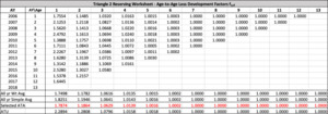
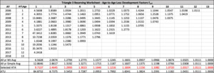
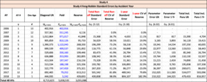
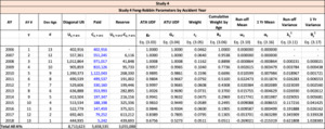
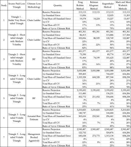
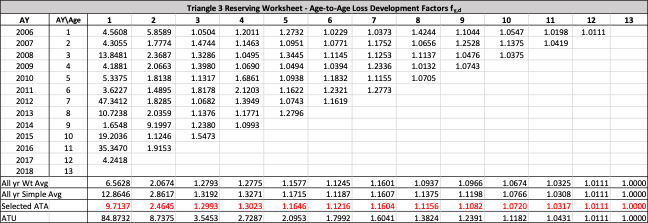
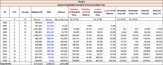
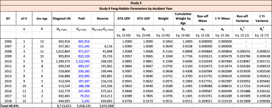
There are seven studies in total. Each study is based upon a particular set of ultimate loss triangles and is evaluated using all of the aforementioned reserve risk methods. Furthermore, each ultimate loss triangle is generated using one of three sets of paid triangles and by applying one of four ultimate loss selection approaches. These approaches include chain ladder, BF, and two hybrid selection methods which we call actuarial best estimate and management booked estimate. The rules for the hybrid selection methods are shown in Appendix C.1, which also derives the ultimate loss triangle from the paid loss triangle and presents all the underlying assumptions. Appendix C.2 presents the worksheets that quantify the reserve risk based on the ultimate loss triangles derived in Appendix C.1.

The following are observations based on a review of the numerical results in Table 23.

• Study 1 is performed using data from Siegenthaler (2019) and produced identical results for the Siegenthaler method, the Mack method and the Merz-Wuthrich method as published in Siegenthaler (2019).

• The Feng-Robbin standard error for total run-off risk is often higher than the Rehman-Klugman result due to the inclusion of additional covariance terms.

• The Feng-Robbin result for one-year risk is often comparable to the Siegenthaler result.

• Compared with the total run-off risk using the Siegenthaler method, the total run-off risk using the Feng-Robbin method is sometimes larger and other times smaller.

• The Feng-Robbin method and the Siegenthaler method usually indicate a lower ratio of one-year CV to total run-off CV than the ratio of Merz-Wuthrich one-year CV to Mack total run-off CV. Lower ratios of one-year CV to total run-off CV are usually appropriate for longer-tailed lines of business, especially when reserves are set using an initial expected loss ratio or the BF method.

• Studies 4 – 7 use the same triangles and demonstrate that reserve risk based on the actuarial central estimate (Study 6) or management booked estimates (Study 7) can be very different from reserve risk assuming reserves are set using a particular method such as chain-ladder (Study 4) or BF (Study 5).

• Study 7 shows that when there is consistent adverse development or consistent favorable development, the Feng-Robbin method yields lower standard error than the Siegenthaler method.

Table 23.Summary of Numerical Results

7.3. Overall Evaluation

The Feng-Robbin method’s treatment of covariance terms is beneficial for evaluating reserve risk because it fully considers the impact of covariance. All of the procedures proposed in this paper eliminate the possibility of negative calculated variance that arises from the triangle structure problem.

In comparison with the Siegenthaler method, both the Feng-Robbin and the Rehman-Klugman methods measure variances of $g_{d}$ factors around their own means, whereas the Siegenthaler method measures variances of $g_{d}$ factors around 1. In the Feng-Robbin method, the deviation of the mean of $g_{d}$ from 1 is captured in the parameter risk.

Both the Feng-Robbin and Siegenthaler methods tend to compute a lower ratio of one-year risk as a portion of total runoff risk than the ratio indicated by the Mack method and the Merz-Wuthrich method. The Mack method and the Merz-Wuthrich method theoretically only apply when reserves are set using the chain-ladder method, whereas the Feng-Robbin method, the Siegenthaler method and the Rehman-Klugman method will be applicable in more general settings.

8. CONCLUSION

This paper has been an exploration into fully accounting for the covariance terms in computing reserve risk based on triangles of estimated ultimate losses. It has expanded the Rehman-Klugman method from the total-run off standard error to a one-year standard error. Procedures were proposed for modifying the covariance matrix to eliminate the possibility of negative calculated variance that arises from the triangle structure problem. A broader examination of the fill-in procedure and its derivatives for analysis of triangle data deserves research of its own. This work points to the need for further investigation into the statistical significance of variance and covariance terms for mature ages. Overall, this paper has attempted to provide readers with additional insights into alternative ways to estimate risk from ultimate loss triangles.

Appendices

Appendix A – TAYLOR SERIES APPROXIMATIONS

Lemma A.1 Using the first-order Taylor Series approximations,

$$\ln\left( \frac{\sum_{y = 1}^{Y}U_{y,\ D}}{\sum_{y = 1}^{Y}U_{y,D - y + 1\ }} \right) \approx \ \sum_{d = 1}^{D}{R_{d}\ln(g_{d})}$$

Proof.

$$\frac{\sum_{y = 1}^{Y}U_{y,D}}{\sum_{y = 1}^{Y}U_{y,D - y + 1\ }} = \ \frac{\sum_{y = 1}^{Y}{U_{i,\ D - y + 1} \times \ G_{D - y + 1}}}{\sum_{y = 1}^{Y}U_{y,\ D - y + 1\ }} = \ \sum_{y = 1}^{Y}{r_{y}G_{D - y + 1}}$$

Taking the logarithm of the ratio above yields

$$\ln\left( \frac{\sum_{y = 1}^{Y}U_{y,\ D}}{\sum_{y = 1}^{Y}U_{y,D - y + 1\ }} \right) = \ln{(\sum_{y = 1}^{Y}{r_{y}G_{D - y + 1}}}) = \ \ln\left( \sum_{y = 1}^{Y}{r_{y} \times e^{\ln\left( G_{D - y + 1} \right)}} \right)$$

Using the first-order Taylor Series approximation $e^{x} \approx 1 + x$ with $x = \ln\left( G_{D - y + 1} \right) \approx 0,$

$$\begin{align} \ln\left( \frac{\sum_{y = 1}^{Y}U_{y,\ D}}{\sum_{y = 1}^{Y}U_{y,D - y + 1\ }} \right) &\approx \ln(\sum_{y = 1}^{Y}r_{y} \times \left\lbrack 1 + \ln\left( G_{D - y + 1} \right) \right\rbrack) \\ &= \ln(\sum_{y = 1}^{Y}r_{y} + \ \sum_{y = 1}^{Y}r_{y}\ln\left( G_{D - y + 1} \right))\\ &= \ln\left( 1 + \ \sum_{y = 1}^{Y}r_{y}\ln\left( G_{D - y + 1} \right) \right) \end{align}$$

Using the first-order Taylor Series approximation $\ln(x) \approx x - 1$ with $x = 1 + \ \sum_{y = 1}^{Y}r_{y}\ln\left( G_{D - y + 1} \right) \approx 1,$

$$\ln\left( \frac{\sum_{y = 1}^{Y}U_{y,\ D}}{\sum_{y = 1}^{Y}U_{y,D - y + 1\ }} \right) \approx \ 1 + \sum_{y = 1}^{Y}r_{y}\ln\left( G_{D - y + 1} \right) - 1$$

$$= \sum_{y = 1}^{Y}r_{y}\ln\left( \prod_{d = D - y + 1}^{D}g_{d} \right) = \sum_{y = 1}^{Y}r_{y}\sum_{d = D - y + 1}^{D}{\ln\left( g_{d} \right)}$$

Substituting $d = D - y + 1,$ and switching the order of summation of $d$ and $y,$ and letting $R_{d} ≔ \sum_{y = D - d + 1}^{Y}{r_{y}\ },$ yields

$$\begin{align} \ln\left( \frac{\sum_{y = 1}^{Y}U_{y,\ D}}{\sum_{y = 1}^{Y}U_{y,D - y + 1\ }} \right) &\approx \sum_{y = 1}^{Y}r_{y}\sum_{d = D - y + 1}^{D}{\ln\left( g_{d} \right)} \\ &= \ \ \sum_{y = 1}^{Y}{\sum_{d = D - y + 1}^{D}{r_{y}\ \ln(g_{d})}} \\ &= \ \ \sum_{d = 1}^{D}{\sum_{y = D - d + 1}^{Y}{r_{y}\ \ln(g_{d})}} \\ &= \ \sum_{d = 1}^{D}{R_{d}\ln(g_{d})} \end{align}$$

Lemma A.2 Using the first-order Taylor Series approximations,

$$\ln\left( \frac{\sum_{y = 1}^{Y}U_{y,D - y + 2}}{\sum_{y = 1}^{Y}U_{y,D - y + 1\ }} \right) \approx \ \sum_{y = 1}^{Y}r_{y}\ln\left( g_{D - y + 1} \right)$$

Proof.

$$\frac{\sum_{y = 1}^{Y}U_{y,D - y + 2}}{\sum_{y = 1}^{Y}U_{y,D - y + 1\ }} = \ \frac{\sum_{y = 1}^{Y}{U_{i,\ D - y + 1} \times \ g_{D - y + 1}}}{\sum_{y = 1}^{Y}U_{y,\ D - y + 1\ }} = \ \sum_{y = 1}^{Y}{r_{y}g_{D - y + 1}}$$

Taking the logarithm of the ratio above yields

$$\ln\left( \frac{\sum_{y = 1}^{Y}U_{y,D - y + 2}}{\sum_{y = 1}^{Y}U_{y,D - y + 1\ }} \right) = \ln{(\sum_{y = 1}^{Y}{r_{y}g_{D - y + 1}}}) = \ \ln\left( \sum_{y = 1}^{Y}{r_{y} \times e^{\ln\left( g_{D - y + 1} \right)}} \right)$$

Using the first-order Taylor Series approximation $e^{x} \approx 1 + x$ with $x = \ln\left( g_{D - y + 1} \right) \approx 0,$

$$\begin{align} \ln\left( \frac{\sum_{y = 1}^{Y}U_{y,D - y + 2}}{\sum_{y = 1}^{Y}U_{y,D - y + 1\ }} \right) &\approx \ln(\sum_{y = 1}^{Y}r_{y} \times \left\lbrack 1 + \ln\left( g_{D - y + 1} \right) \right\rbrack) \\ &= \ln(\sum_{y = 1}^{Y}r_{y} + \ \sum_{y = 1}^{Y}r_{y}\ln\left( g_{D - y + 1} \right)) \\&= \ln\left( 1 + \ \sum_{y = 1}^{Y}r_{y}\ln\left( g_{D - y + 1} \right) \right) \end{align}$$

Using the first-order Taylor Series approximation $\ln(x) \approx x - 1$ with $x = 1 + \ \sum_{y = 1}^{Y}r_{y}\ln\left( g_{D - y + 1} \right) \approx 1,$

$$\begin{align} \ln\left( \frac{\sum_{y = 1}^{Y}U_{y,D - y + 2}}{\sum_{y = 1}^{Y}U_{y,D - y + 1\ }} \right) &\approx \ 1 + \sum_{y = 1}^{Y}r_{y}\ln\left( g_{D - y + 1} \right) - 1 \\ &= \sum_{y = 1}^{Y}r_{y}\ln\left( g_{D - y + 1} \right) \end{align}$$

Appendix B – MATRIX THEORY

Definition B.1 Let $\mathbf{M}$ be an $n \times n$ symmetric real-valued matrix, and $\overrightarrow{v}$ be a $n \times 1$ real-valued column vector. Matrix $\mathbf{M}$ is positive semi-definite if and only if ${\overrightarrow{v}}^{T}\mathbf{M}\overrightarrow{v} \geq 0$ for all possible values of $\overrightarrow{v}.$

Theorem B.2 Let $\mathbf{M}$ be an $n \times n$ matrix. A) if $\mathbf{M}$ is a valid covariance matrix with no missing data, then $\mathbf{M}$ is positive semi-definite. B) If $\mathbf{M}$ is positive semi-definite, then M is a valid covariance matrix of $n$ random variables.

Proof. See Stefanica [16] Theorem 7.5 part (i). Intuitively this theorem makes sense, as the product ${\overrightarrow{v}}^{T}\mathbf{M}\overrightarrow{v}$ is the variance of the linear combination of $n$ random variables with coefficients vector $\overrightarrow{v},$ and the computed variance should always be non-negative regardless the values of coefficients in $\overrightarrow{v}.$

Lemma B.3 Let $\mathbf{X}$ be an$\ n \times n$ diagonal matrix with non-negative real numbers on the diagonal and zero everywhere else. Then $\mathbf{X}$ is positive semi-definite.

Proof. Let$\ \overrightarrow{v} = {(v_{1}\ v_{2}\ldots\ v_{n})}^{T}$ be an arbitrary $n \times 1$ real-valued vector. Denote the diagonal elements of matrix $\mathbf{X}$ by $x_{1},$ $x_{2},$ … $x_{n}$ where each element is non-negative. Because $\mathbf{X}$ is a diagonal matrix, ${\overrightarrow{v}}^{T}\mathbf{X}\overrightarrow{v} = \ \sum_{i = 1}^{n}{v_{i}^{2}x_{i}} \geq 0.$ This satisfies Definition B.1 for $\mathbf{X}$ to be positive semi-definite.

Lemma B.4 Let $\mathbf{M}$ and $\mathbf{P}$ be positive semi-definite matrices of the same dimension. Then $\mathbf{M + P}$ is positive semi-definite.

Proof. Let$\ \overrightarrow{v} = {(v_{1}\ v_{2}\ldots\ v_{n})}^{T}$ be an arbitrary $n \times 1$ real-valued vector. Because $\mathbf{M}$ and $\mathbf{P}$ are positive semi-definite, ${\overrightarrow{v}}^{T}\mathbf{P}\overrightarrow{v} \geq 0$ and ${\overrightarrow{v}}^{T}\mathbf{M}\overrightarrow{v} \geq 0.$ Then, ${\overrightarrow{v}}^{T}\left( \mathbf{P + M} \right)\overrightarrow{v} = {\overrightarrow{v}}^{T}\mathbf{P}\overrightarrow{v} + {\overrightarrow{v}}^{T}\mathbf{M}\overrightarrow{v} \geq 0.$ This satisfies Definition B.1 for $\mathbf{P + M}$ to be positive semi-definite.

Lemma B.5 $\mathbf{M}_{Diag}$ is positive semi-definite.

Proof. Define a diagonal matrix $\mathbf{P}$ that has a diagonal that is equal to the diagonal of the nominal covariance matrix $\mathbf{N}$ subtract the diagonal of the fill-in covariance $\mathbf{M}_{fill - in}.$ The $d$-th diagonal of matrix $\mathbf{P}$ is given by $\mathbf{P}_{dd} = \mathbf{N}_{dd} - \mathbf{M}_{fill - in,\ \ \ dd}.$ Then, $\mathbf{M}_{Diag} = \mathbf{M}_{fill - in} + \mathbf{P}\ .$ It suffices to demonstrate that elements of $\mathbf{P}$ are non-negative. If so, Lemma B.3 and Theorem B.2 prove $\mathbf{P}$ and $\mathbf{M}_{fill - in}$ are positive semi-definite, and it follows from Lemma B.4 that $\mathbf{M}_{Diag}$ is also positive semi-definite.

$$\begin{align} \mathbf{M}_{fill - in,\ \ \ dd} &= \ \frac{\sum_{y = 1}^{Y - d}{{{(ln(g}_{y,d}) - {\widehat{\mu}}_{d})}^{2} + \sum_{y = Y - d + 1}^{Y - 1}{{({\widehat{\mu}}_{d} - {\widehat{\mu}}_{d})}^{2}\ }}}{Y - 2} \\ &= \frac{\sum_{y = 1}^{Y - d}{{{(ln(g}_{y,d}) - {\widehat{\mu}}_{d})}^{2}\ }}{Y - 2} \leq \frac{\sum_{y = 1}^{Y - d}{{{(ln(g}_{y,d}) - {\widehat{\mu}}_{d})}^{2}\ }}{Y - d - 1} \\ &= \mathbf{N}_{dd} = \mathbf{M}_{Diag,\ dd}. Therefore, \mathbf{P}_{dd} \geq 0. \end{align}$$

Theorem B.6 Let $\mathbf{M}$ be an $n \times n$ real valued matrix. $\mathbf{M}$ is positive semi-definite if and only if there is another $n \times n$ matrix real valued matrix $\mathbf{P}$ such that $\mathbf{M =}\mathbf{P}^{T}\mathbf{P}$

Proof. See Horn and Johnson [6] Theorem 7.2.7 part (a). Note that the Horn and Johnson proof applies to more general complex-valued matrices while this paper is restricted to real valued matrices. This theorem will be used to prove Lemma B.7 below.

Lemma B.7 If $n \times n$ matrices $\mathbf{M}$ and $\mathbf{P}$ are positive semi-definite, then the matrix product $\mathbf{P}^{T}\mathbf{MP}$ is also positive semi-definite.

Proof. According to Theorem B.3, there exist $n \times n$ matrices $\mathbf{A}$ and $\mathbf{B}$ such that $\mathbf{M =}\mathbf{A}^{T}\mathbf{A}$ and$\mathbf{\ P =}\mathbf{B}^{T}\mathbf{B}.$ Then, $\mathbf{P}^{T}\mathbf{MP =}{\mathbf{(B}^{\mathbf{T}}\mathbf{B)}}^{T}\mathbf{(A}^{\mathbf{T}}\mathbf{A)}\mathbf{(B}^{\mathbf{T}}\mathbf{B) =}\mathbf{B}^{T}\mathbf{B}\mathbf{A}^{T}\mathbf{A}\mathbf{B}^{T}\mathbf{B =}\left( \mathbf{A}\mathbf{B}^{T}\mathbf{B} \right)^{T}\mathbf{(A}\mathbf{B}^{T}\mathbf{B)},$ and applying Theorem B.6 backward implies that $\mathbf{P}^{T}\mathbf{MP}$ is also positive semi-definite.

Lemma B.8 $\mathbf{M}_{full} = \mathbf{X}^{T}\mathbf{M}_{fill - in}\mathbf{X}$ is positive semi-definite.

Proof. Theorem B.2 and Lemma B.3 establish that $\mathbf{M}_{fill - in}$ and$\mathbf{\ X}$ are positive semi-definite, respectively. Applying Lemma B.7 yields that $\mathbf{M}_{full}$ is also positive semi-definite.

Lemma B.9 The $d$-th diagonal of $\mathbf{M}_{full} = \mathbf{X}^{T}\mathbf{M}_{fill - in}\mathbf{X}$ is equal to the raw sample variance of the corresponding age in the triangle of $ln(g_{d}),$ ${{\widehat{\sigma}}_{d}}^{2}$

Proof. Denote the $d$-th element in the diagonal of matrix $\mathbf{M}_{fill - in}$ as $m_{d}.$ Denote the $d$-th element in the diagonal of matrix $\mathbf{X}$ as $x_{d}.$ The $d$-th element in the diagonal of matrix $\mathbf{M}_{full} = \mathbf{X}^{T}\mathbf{M}_{fill - in}\mathbf{X}$ is calculated by $x_{d}^{2}m_{d}.$ The calculation is simplified significantly because matrix $\mathbf{X}$ is a diagonal matrix. Recall from Section 5.2.3 that

$$x_{d} = \ \left\{ \begin{matrix} \sqrt{\frac{D - 2}{D - d - 1}}\ \ \ if\ d \leq D - 2 \\ 0\ \ \ \ \ \ \ \ \ \ \ \ \ \ \ \ \ \ \ \ otherwise \\ \end{matrix} \right.\ $$

If $d \leq D - 2,$ random variable $\ln(g_{d})$ has $D - d$ samples in the triangle of $ln(g_{d}).$ The sample mean and variance of $ln(g_{d})$ is given by:

$${\widehat{\mu}}_{d} = \ \frac{\sum_{y = 1}^{Y - d}{{\ln(g}_{y,d})\ }}{Y - d}$$

$${{\widehat{\sigma}}_{d}}^{2} = \ \frac{\sum_{y = 1}^{Y - d}{{{(\ln(g}_{y,d}) - {\widehat{\mu}}_{d})}^{2}\ }}{Y - d - 1}$$

The fill-in procedure in Section 5.2.1 supplants the triangle of $ln(g_{d})$ with ${\widehat{\mu}}_{d}$ for each age $d$ to complete the square. The mean of the new “filled-in square” of $ln(g_{d})$ is obviously still ${\widehat{\mu}}_{d}.$ The variance of the new “filled-in square” of $ln(g_{d})$ is the $d$-th element in the diagonal of matrix $\mathbf{M}_{fill - in},$ $m_{d},$ and is given as

$$\begin{align} m_{d} &= \ \frac{\sum_{y = 1}^{Y - d}{{{(\ln(g}_{y,d}) - {\widehat{\mu}}_{d})}^{2} + \sum_{y = Y - d + 1}^{Y - 1}{{({\widehat{\mu}}_{d} - {\widehat{\mu}}_{d})}^{2}\ }}}{Y - 2} \\ &= \frac{\sum_{y = 1}^{Y - d}{{{(\ln(g}_{y,d}) - {\widehat{\mu}}_{d})}^{2}\ }}{Y - 2} \end{align}$$

To complete the proof,

$$\begin{align} x_{d}^{2}m_{d} &= \frac{Y - 2}{Y - d - 1} \times \frac{\sum_{y = 1}^{Y - d}{{{(\ln(g}_{y,d}) - {\widehat{\mu}}_{d})}^{2}\ }}{Y - 2} \\ &= \ \frac{\sum_{y = 1}^{Y - d}{{{(\ln(g}_{y,d}) - {\widehat{\mu}}_{d})}^{2}\ }}{Y - d - 1} = {{\widehat{\sigma}}_{d}}^{2} \end{align}$$

Appendix C – EXHIBITS FOR NUMERICAL EXAMPLES

This appendix provides the exhibits for numerical examples. From 3 sets of paid triangles, Appendix C.1 derives seven ultimate loss triangles used in each of the 7 reserve risk studies. The relationships between the studies and the source triangles are laid out in the following table:

In Appendix C.2, an example of reserve risk worksheet for the Feng-Robbin method, the Rehman-Klugman method, the Siegenthaler method, the Mack method, and the Merz-Wuthrich method for Study 4 is presented. Other Studies were generated using identical worksheets and the full exhibits is available online.

C.1 Reserving Worksheets

 

 

 

 

 

 

 

 

 

 

 

 

 

 

 

 

 

 

C.2 Risk Worksheets (Study 4 Only)

In the worksheets for the Feng-Robbin method, the Rehman-Klugman method, and the Siegenthaler method, the only required inputs are the ultimate loss triangle and latest diagonal of paid loss (in blue text). In the worksheet for the Mack method and Merz-Wuthrich method, the only required input is the paid loss triangle (in blue text).