The LaPlace Transform as Stochastic Present Value

undefined

1. INTRODUCTION

As we enter a period of rising interest rates, it is a good time to consider extending our view of present value to make it stochastic. This paper will present for an actuarial audience the idea that stochastic present value is given by the LaPlace transform. Of equal importance is the converse statement, that we can attach a meaning to the transform in a financial context.

The topic of present value is central to actuarial science. Insurance policies typically exchange a fixed payment at policy inception for an uncertain stream of payments at later dates. We currently have a deterministic view of present value that disregards the stochastic nature of interest rates and cash flow amounts.

The idea of the LaPlace transform as stochastic present value has appeared in finance journals since 1967 (Grubbström 1967). We have no other formula for stochastic present value, so “proving” their equivalence amounts to demonstrating that the LaPlace transform is a suitable candidate. So, the purpose of this paper is not to prove it rigorously, but to familiarize readers with the transform.

One advantage to using the LaPlace transform is that it allows us to model cyclical variations in the trend of the time value of money. The LaPlace transform can be described as a method of finding the cyclical patterns around an exponential trend. Economic cycles drive interest rate cycles, and the LaPlace transform allows us to simultaneously find both the dominant trend and the economic cycle in the data. These cycles are important because they constitute systemic risk in simple exponential models.

A second advantage of the LaPlace transform is that it allows us to model stochastic cash flows, while discounting them in the same formula. Any stochastic process can be described by its Fourier transform, which is a special case of the LaPlace transform. In particular, the cash flow distribution can be represented by its LaPlace transform.

There are several practical impediments to the use of the LaPlace transform in actuarial science; we lack a physical interpretation of the transform, it requires a change in perspective to a frame of reference that we seldom use, and it involves complex arithmetic. This paper will define terms and provide interpretations and visualizations of the transform, the alternate frame of reference, and the meaning of complex values in an actuarial setting.

1.1. Research Context

Stochastic present value was most recently addressed by Leigh Halliwell in 2003 (Halliwell 2003). Halliwell argues that stochastic present value is a distribution, but decision making requires a single value, so a utility function is needed to resolve the distribution to a number. In Halliwell’s view, utility functions are subjective, so we must ultimately turn to the marketplace to resolve questions of value.

The LaPlace transform has not been directly associated with stochastic present value in the CAS literature. Insurance applications of the LaPlace transform in a present value context have appeared in several papers by European academics. M.J. Gooverts and Ann De Schepper have used the transform in several papers on annuities (De Schepper, De Vylder, and Goovaerts 1992; De Schepper and Goovaerts 1992; De Schepper, Teunen, and Goovaerts 1994). They also applied it in the non-life world with “IBNR Reserves Under Stochastic Interest Rates” (Goovaerts and De Schepper 1997), but loss reserve discounting is narrowly constrained in U.S. statutory accounting, and the paper does not seem to have attracted much attention.

In a 1967 paper in Management Science, Robert Grubbström showed that the present value formula and the LaPlace transform agree precisely for deterministic cash flows and agree in the mean for stochastic cash flows and/or interest rates. Grubbström went on to propose the adoption of the LaPlace transform in finance because the transform is also useful for the solution of differential equations and convolution equations. This last point is of particular importance in an actuarial context since convolution equations occur naturally in loss reserving, as developed by Ira Robbin (Robbin 2004).

In 1986, Stephen A. Buser published a note in the Journal of Finance entitled “LaPlace Transforms as Present Value Rules.” Buser gives a very concise demonstration of the link between present value and the LaPlace Transform:

"One of the recurring problems in finance is to find the present value of a given cash flow C(t) for a given rate of discount r.

$$V(r) = \int_{0}^{\infty}{e^{- rt}C(t)dt}\tag{1.1}$$

In standard mathematical jargon, the present value integral, V(r), is referred to as the LaPlace transform of the cash flow, C(t)."

Buser’s argument is concise, but it hides the fact that it introduces a change to the meaning of the variable r. We normally think of present value as a function of the discount rate, but in the LaPlace transform the variable r is allowed to take complex values. The real part of r can be described as a discount rate, but the imaginary part is interpreted as a frequency. There should be no surprise that we would have to add a term to make present value stochastic. The real variable r has been implicitly replaced by a complex variable.

Buser’s motivation was to gain access to the tabular results for the LaPlace transform for their application in finance problems. Buser’s paper includes a transform table, some excerpts of which are shown in the table below. When the LaPlace transform is considered as an operator acting on functions it is often denoted by $\mathcal{L\lbrack}f\rbrack$, but when it is considered as a function of r, the transform of $f(t)$ is denoted by $F(r)$.

The table above includes a function denoted $\delta(t)$, known as the delta function, which as a distribution represents a point mass at time t=0. Similarly, $\delta(t - t_{0})$ denotes a point mass at time t₀.

Each of the cases above describes a deterministic cash flow. It should be no surprise that the LaPlace transform agrees with the known present value for the distribution, given that the two formulas agree. The reason that I included this table is to reinforce the fact that the LaPlace transform agrees our familiar idea of present value for deterministic cash flows.

Transform tables typically include more than just the transforms of simple functions, they also include entries that depict the response of the transform to operations on the input function.

These operations speak to Grubbström’s motivation; they allow us to perform calculations that might otherwise be difficult. If we equate the LaPlace transform with stochastic present value, then each of these operations becomes available to us. Working in present values lets users find moments, shift the input distribution or the output distribution, take derivatives, integrate, and add distributions using the LaPlace transform rules. Time-shifted input distributions are of particular interest in loss reserving, where time-shifting may be used to describe report lags and/or payment lags (Robbin 2004).

Nothing in this paper should be construed as advocating for stating reserves at present values. However, I am suggesting that it may be advantageous at times to do calculations with present values and then transform back to nominal values. The process of transforming to a convenient basis, calculating, then transforming back, should be familiar to actuaries: we use this approach with log-linear regression models.

1.2. Objective

The objectives of this paper are to familiarize actuaries with the LaPlace transform and to give a formula for stochastic present value. While we have an idea of the meaning of stochastic present value, we currently lack a formula to compute it. We have the opposite problem with the LaPlace transform, we lack a financial interpretation of the formula. Equating the two gives us a formula for stochastic present value and an example of the LaPlace transform.

The scope of this paper will be limited to the use of the LaPlace transform as present value to maintain clarity. However, the transform has other potential uses. For example, the formula for bringing losses to a common cost basis takes the same form as the present value formula, with deflating replacing discounting. In other words, modeling inflation is another possible application of the LaPlace transform in actuarial science, but it will not be specifically addressed here.

With the limited scope, the purpose of this paper is to establish a precedent for the use of the LaPlace transform other than in the calculation of aggregate loss distributions. In future work, I intend to use the LaPlace transform in applications involving inflation once the precedent is established. I chose to focus on present value, rather than inflation, because the precedent already exists in finance.

In mathematics, generality is favored over specific examples. It is left up to practitioners to interpret the meaning of mathematical objects as they appear in each discipline. So it is with the LaPlace transform in actuarial science. Mathematicians have developed a powerful tool supported by rigorous theory, but we rarely use it. This is in part because we don’t have an interpretation of its meaning in our world. To remedy this, I am providing my own interpretations of the LaPlace transform in an actuarial setting.

1.3. Outline

This paper will provide a series of examples and visualizations to introduce the LaPlace transform to actuaries who might not have previously encountered it. For the LaPlace transform to serve as stochastic present value it must accommodate stochastic interest rates, stochastic cash flows, and it must be understandable.

The remainder of the paper addresses these requirements as follows. Section 2 will provide helpful background material. Section 3 illustrates graphically how the LaPlace transform models variations in rates. Section 4 then gives examples to show how the LaPlace transform can model stochastic cash flow amounts. Finally, section 5 describes the Discrete Fourier Transform and briefly outlines how it works.

2. Background Materials

The LaPlace transform is usually associated with the study of wave phenomena in a physical or electromagnetic setting. In a financial environment, business cycles are associated with cycles in interest rates and cash flow amounts. Using the LaPlace transform for stochastic present value means that we are going to treat the business cycle effects as waves.

The challenge with visualizing stochastic present value is that it allows both interest rates and cash flows to vary. We can simplify the problem by holding one of these two factors fixed. This will be done by introducing the Fourier transform to model stochastic cash flow amounts. The Fourier transform is a special case of the LaPlace transform, it models distributions with waves, but it lacks a discount factor.

2.1. Waves

A function that satisfies the equation $f(x + T) = f(x)$ is known mathematically as a periodic function, with period $T$. The physical manifestation of periodic phenomena is referred to as a wave or waves. Ocean waves give us a visualization of a periodic function; it is a natural process that repeats itself at regular or semi-regular intervals. The visually intuitive term wave has become almost synonymous with the mathematically descriptive term periodic function.

Waves are often described in terms of their amplitude and wavelength. Amplitude can be thought of as the height of a wave, measured at its highest point. In physical settings the term wavelength is used to mean the period, or the time between wave crests. The following graph gives a visual representation of amplitude and wavelength:

The term harmonic is used for a simple wave of the form:

$$y = A\ sin(\omega t + \theta)\tag{2.1}$$

The maximum height or trough of the wave is called the amplitude. It is given by $|A|$.

The frequency $\omega = \frac{1}{wavelength}$ gives the number of wave crests in a fixed period of time.

The phase $\theta$ has the effect of shifting the entire wave forward or backwards in time. For example, $\cos(t) = sin(t + \frac{\pi}{2})$ describes the cosine as a shifted sine function.

2.2. Complex numbers

The mathematics of waves is usually done using complex arithmetic. We will need to know a little about complex numbers to understand and interpret the LaPlace transform.

A number $s$ is said to be a complex number if it can be expressed in the form

$s = \alpha + i\omega$, where $\alpha$ and $\omega$ are real numbers, and $i = \sqrt{- 1}$.

$\alpha$ is referred to as the real part of $s$, while $i\omega$ is referred to as the imaginary part. If $\alpha = 0$ we say that $s$ is purely imaginary.

The complex conjugate of $s = \alpha + i\omega$ is denoted by $\overline{s}$, with $\overline{s} = \alpha - i\omega$.

The product of a complex number with its complex conjugate returns a positive real number. Readers should be able to work out for themselves that:

$$s\ \overline{s} = \alpha^{2} + \omega^{2}\tag{2.2}$$

The absolute value of a complex number is given by:

$$|s| = \sqrt{s\overline{s}}\tag{2.3}$$

Functions with complex exponents produce complex waves. We should all be familiar with Euler’s formula:

$$e^{ix} = \cos x + i\sin x\tag{2.4}$$

Real valued harmonic functions can be represented as sums of complex exponentials. The basic trigonometric functions are produced by

$$\cos x = \frac{e^{ix} + e^{- ix}}{2}\tag{2.5}$$

and

$$\sin x = \frac{e^{ix} - e^{- ix}}{2i}\tag{2.6}$$

2.3. Modeling Distributions as waves

There is a perspective in statistics that views time series data as observations of wave processes. This view is described in section 3.6 of Emmanual Parzen’s textbook entitled “Stochastic Processes” (Parzen 1967). In this framework the time series data is interpolated with a series of harmonic functions. The details of the interpolation process appear in section 5, but for now I want to focus on the frame of reference of this time series/wave point of view.

We occasionally take this time series/wave point of view in casualty actuarial science. When talking about catastrophic events such as earthquakes, floods, and large hurricanes, we use idea of return time, e.g., a 100 year storm. Return time is a measure of the time between events, i.e., it is a wavelength. The reciprocal of return time is an excess frequency. In this view of catastrophic events, we think of annual losses as a time series, while large deviations from the norm (catastrophic events) are expressed in terms of their excess frequency. When expressed as a wave, the amount of the deviation from the mean is the amplitude, and the excess frequency is the wave frequency.

This example is relevant to our discussion of stochastic present value because aggregate loss payment distributions are the most interesting stochastic insurance cash flows. When we model aggregates loss payments, we might phrase an estimate in terms such as “The probability of $X million in payments next year is Y%.” The amount of payment is the domain, and the range is a probability.

Some insurance questions require us to reverse the domain and the range. In capitalization questions we may ask “how much capital do we need for a 1% risk of failure?” Notice that frequency is now the domain (1% per year), while the range is an amount (how much capital). In this sense, frequency and probability have a similar meaning. Probability expresses the relative frequency of occurrence. Probability is expressed as the rate of successes per trial, so it is restricted to values from zero to one. Frequency is the rate of occurrences per time period, so it may take values greater than one. Probabilities are frequencies, but frequencies are not necessarily probabilities.

The Fourier transform changes perspective from frequency by amount to amount by frequency. There are both continuous and discrete forms of the Fourier transform. The continuous form transforms a probability density function to its wave representation, while the discrete form finds the coefficients to interpolate time series data with a series of waves. I have placed the Discrete Fourier Transform at the end of paper because this paper is not about a specific application, but I have included it because I believe that we actuaries can visualize the interpolation concept more easily than we can decipher the continuous formula. We will use the continuous version for comparison with the LaPlace transform.

2.4. The Fourier Transform

A rigorous treatment of the Fourier and LaPlace transforms is given in A.H. Zemanian’s text entitled “Distribution Theory and Transform Analysis” (Zemanian and Gillis 1965). In section 7.2, Zemanian defines the Fourier transform as:

$$\widetilde{f}(\omega) = \int_{- \infty}^{\infty}{f(x)e^{- i\omega x}dx}\tag{2.6}$$

This formula is similar in form to the present value in formula 1. In this section I will examine the differences. Each of these variations is significant in understanding the meaning of the formula.

The variable x has replaced t in the present value formula. This is a generalization. Present value is a function of time. While the Fourier transform may act on a distribution in time, it is not necessarily time.

Until now, the limits on all the integrals have been 0 to $\infty$, while in general the LaPlace and Fourier transforms are defined with limits of integration that go from $- \infty$ to $\infty$. What we have seen so far is known as the one-sided version of the LaPlace transform. The one-sided version is often used when all the functions involved have positive support, i.e., $f( - t) = 0$ for all $t$. This is the case with present value, where it is assumed that all cash flows occur at $t \geq 0$.

The most significant change is the explicit inclusion of an imaginary number in the exponential term. In the present value formula r is a real number. When we consider an exponential of the form $e^{- rt}$, we interpret r as a discount rate or a rate of decay. However, the complex exponential $e^{- i\omega t}$ describes a complex wave with frequency $\omega$. Substituting $\omega t$ for $x$ in Euler’s equation we get:

$$e^{i\omega t}= \cos(\omega t) + i\ \sin(\omega t)\tag{2.7}$$

This is a complex wave in which $\omega$ is the frequency.

This is a long-winded way of saying that a real valued parameter in an exponential function is interpreted as a rate, while an imaginary valued parameter is interpreted as a frequency. This distinction between rate and frequency is critical because a rate determines discount, while frequencies determine the cyclicality of the discount rate.

To address stochastic cash flows, I think that it is generally understood that any distribution can be uniquely determined by its characteristic function. The Fourier transform and the characteristic function are closely related. Showing the nature of the relationship should make it clear that the Fourier transform also uniquely determines distributions.

Klugman, Panjer and Willmot (2008) give the characteristic function in Definition 6.18 as:

$$\varphi_{X}(z) = E\left( e^{izX} \right) = E(\cos{zX} + i\sin{zX)}\tag{2.8}$$

We can write the expectation as an integral,

$$\varphi_{X}(z) = \int_{- \infty}^{\infty}{f(x)(\cos{zx} + i\sin{zx})dx}\tag{2.9}$$

We can split $\varphi_{X}(z)$ into real and imaginary parts:

$$\varphi_{X}(z) = \int_{- \infty}^{\infty}{f(x)\cos{zx}\ dx + i\int_{- \infty}^{\infty}{f(x)\sin{zx}\ dx}}\tag{2.10}$$

To compare this to the Fourier transform, we can expand equation 2.6 using Euler’s formula, and split the result into real and imaginary parts:

$$\widetilde{f}(\omega) = \int_{- \infty}^{\infty}{f(x)\cos{( - \omega x)}dx + i\int_{- \infty}^{\infty}{f(x)\sin{( - \omega x)}\ dx}}\tag{2.11}$$

We can now restate this using the relationships $\cos{( - x) = \cos x}$ and $\sin{( - x)} = - \sin x$:

$$\widetilde{f}(\omega) = \int_{- \infty}^{\infty}{f(x)\cos{(\omega x)}dx - i\int_{- \infty}^{\infty}{f(x)\sin{(\omega x)}\ dx}}\tag{2.12}$$

Comparing equations 2.12 and 2.10, the Fourier transform is the complex conjugate of the characteristic function. The complex conjugate of a function is unique, so if the characteristic function uniquely determines distributions, the Fourier transform does as well.

In this section we have seen that any distribution can be expressed as its Fourier transform, which takes the same general form as the LaPlace transform. The Fourier transform can be used to model stochastic cash flows, but it has no discount factor. The parameter in the exponential term is purely imaginary, so it should be considered as a frequency rather than a rate.

2.5. The LaPlace transform

Zemanian (1965) defines the LaPlace transform as:

$$\mathcal{L}\left\lbrack f(t) \right\rbrack = \int_{- \infty}^{\infty}{{f(t)e}^{- st}dt}\tag{2.13}$$

The variable $s$ is explicitly defined to be a complex number. We can say $s = \alpha + i\omega$, where $\alpha$ and $\omega$ are real numbers. In this case $\alpha$ can be interpreted as a discount rate, while $\omega$ is a frequency.

We can expand the LaPlace transform formula to explicitly separate the real and complex parts of the exponential:

$$\mathcal{L}\left\lbrack f(t) \right\rbrack = \int_{- \infty}^{\infty}{{f(t)e}^{- \alpha t}e^{- i\omega t}dt}\tag{2.14}$$

The LaPlace transform expresses the distribution of cash flows in terms of waves, while simultaneously discounting. If $\omega = 0$ then this becomes deterministic present value with discount rate $\alpha$. If $\alpha = 0$ then this becomes the Fourier transform $\widetilde{f}(\omega)$. The most important problem is when neither $\alpha$ nor $\omega$ are zero, in which case we could let $g(t) = f(t)e^{- \alpha t}$ and equation 2.14 become:

$$\mathcal{L}\left\lbrack f(t) \right\rbrack = \int_{- \infty}^{\infty}{g(t)e^{- i\omega t}dt}\tag{2.15}$$

or,

$$\mathcal{L}\left\lbrack f(t) \right\rbrack = \widetilde{g}(\omega)\tag{2.16}$$

If $f(t)$ is a stream of cash flows, then we can interpret the LaPlace transform as the Fourier transform of the discounted cash flows.

The behavior of the LaPlace transform in a present value context is illustrated graphically in the sections that follow. They will consider two special cases. In section 3, the cash flows are assumed to be fixed, but interest rates exhibit cyclical variations over time. In section 4, the cash flows are allowed to vary, while interest rates are held fixed.

3. Stochastic Rates

For many actuaries, our standard view of compound interest is that the cumulative value of a risk-free investment increase exponentially over time. This view works quite well during periods of stable interest rates, but its deficiencies become obvious when interest rates vary.

If we take a long-term view of interest rates, we will see that the cumulative value of the amount invested grows slowly during periods of low rates, increases rapidly during a period of high rates, before reaching the next plateau in the cycle.

One way to model this stair-stepped progression of the value of money is to view variable interest rates as a wave around an exponential curve. If the exponent has both real and imaginary terms, it describes a cycle around the trend:

$$e^{t(\alpha + i\beta)} = e^{t\alpha}(\cos{\beta t} + i\sin{\beta t})\tag{3.1}$$

Compound interest can be made to be stochastic by considering the variation in rates as causing waves around an exponential curve. This is illustrated in the graph below:

A complex wave represents both the trend and the cycle as exponentials. Sums of complex exponentials with a common rate can produce a real valued function that cycles around an exponential curve (from equations 2.5 and 2.6).

3.1. Example: U.S. Short Term Interest Rates

To demonstrate the idea of a trend with a cycle, I obtained historical three-month T-Bill rates from the NY Fed website. These yield rates are shown in the following graph, whose standout feature is the historic interest rate peak of the early 1980s:

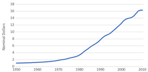
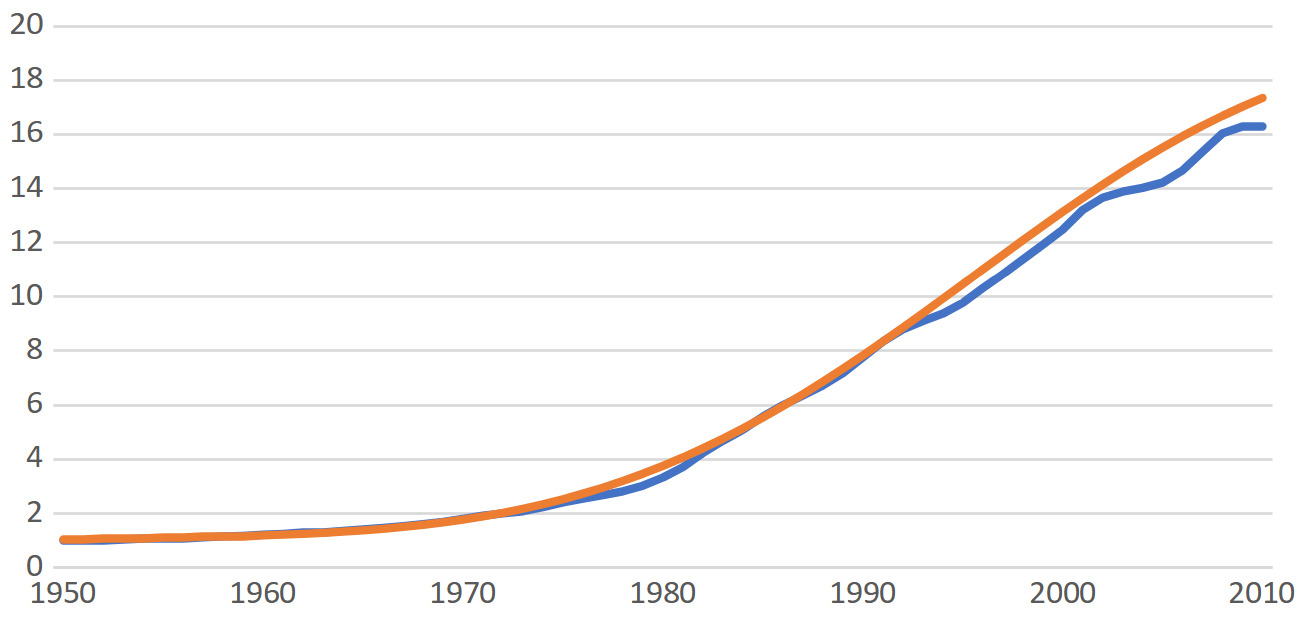
I then constructed an index that depicts the value of $1 continuously reinvested in three-month T-Bills. A graph of this index is shown below:

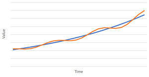
It would be standard actuarial practice to fit an exponential curve to the index:

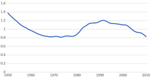
In this typical presentation, we might have some concern that the deviation of the fit from the index is greatest in the most recent years. However, if we look instead at the proportional deviation of the fit from the index, a very clear cyclical pattern emerges:

This cyclical component begs to be fit with a trig function, which we can do by including a complex term (or terms) in our exponential function:

This fit is a real valued function that is the product of an exponential and a cosine. It can be represented as a sum of complex exponentials with two non-zero frequencies. With additional terms the series will fit more closely, until it interpolates the data. The LaPlace transform finds all the terms of the interpolating series with the addition of a single term to the present value formula. This makes it suitable for solving the problem of defining present value in a stochastic rate environment.

There are other possible methods for modeling varying rates. For example, in the context of inflation, Dave Core has demonstrated the use of splines. One advantage of the LaPlace transform is that it allows us to easily perform other operations such as convolutions. Another is that it retains the basic form of the present value formula. In contrast, the use of a spline does not require a change in perspective, which could make it easier to incorporate into existing systems.

4. Stochastic Cash Flow Amounts

In the previous section we saw that a wave cycling around an exponential trend can represent the cyclical patterns in interest and discount rates over time. But we also must consider the problem that the amounts are stochastic. This is the insurance problem: how to determine the present value of stochastic future losses.

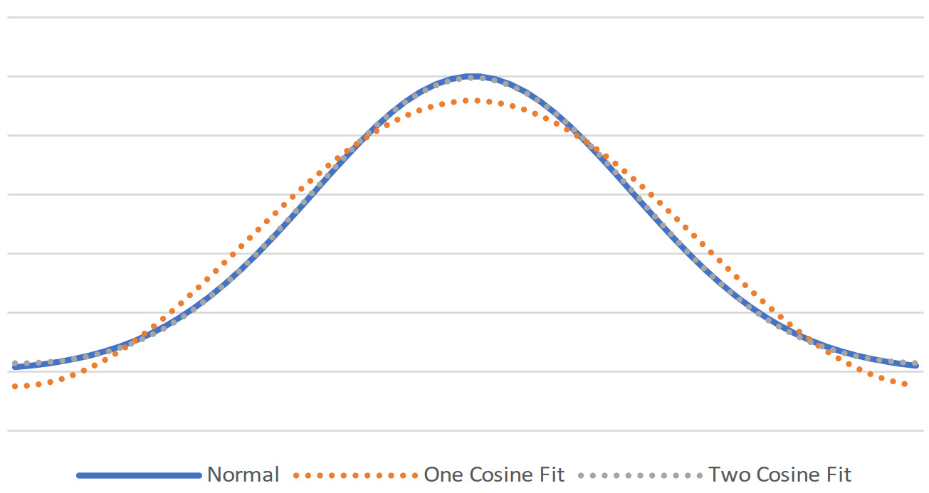
To show that it is plausible to fit familiar distributions with waves, I would like to start with two examples that illustrate familiar distributions interpolated with series of harmonics.

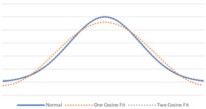
The following graph depicts partial sums of a series of cosines that converge to a Normal distribution centered at the origin:

The two-cosine fit is virtually indistinguishable from the Normal. The cosine series converges very quickly to the Normal PDF because both are even functions, i.e., they only have even terms in their Taylor expansions, so we gain two orders in accuracy for each term added to the cosine series.

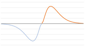
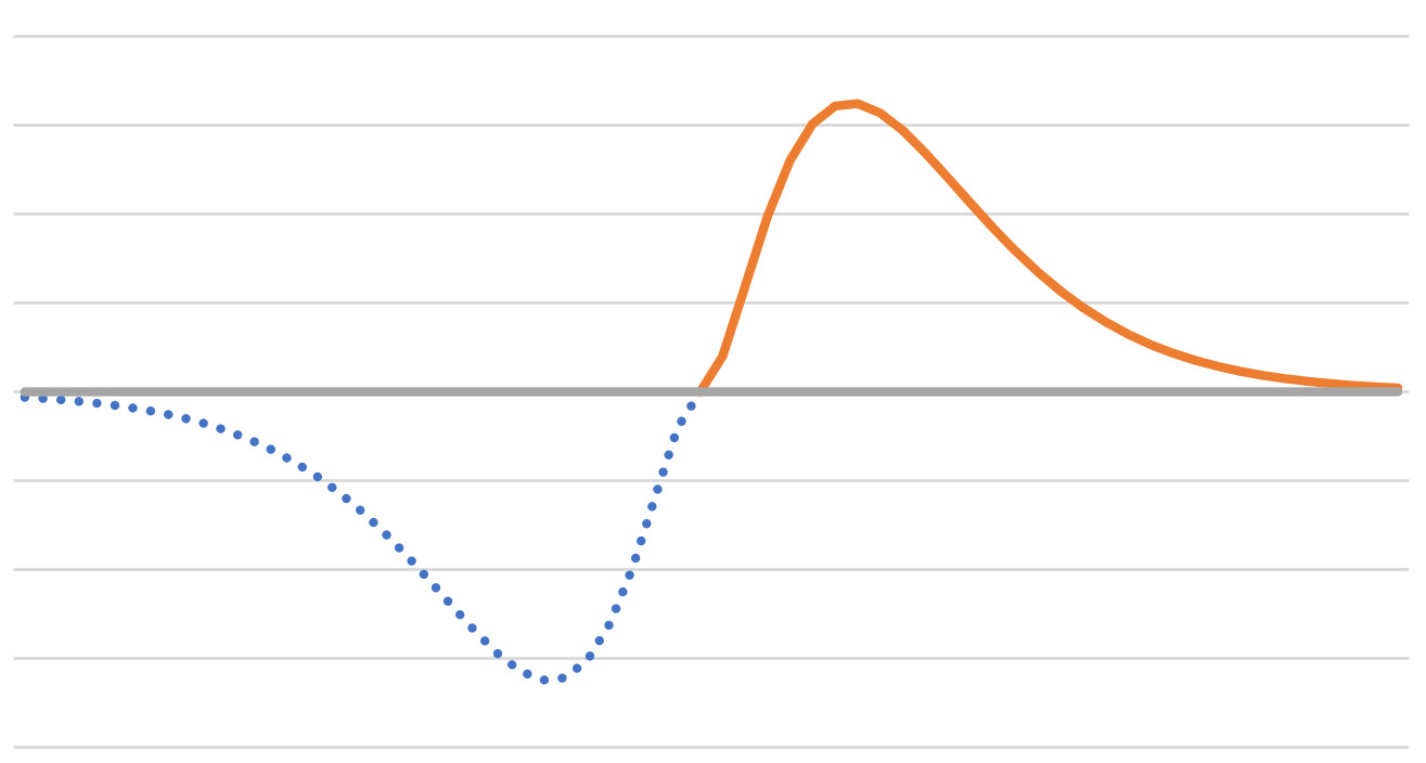
For a contrasting example, consider a Gamma distribution with $f(0) = 0$. It is skewed, so you might think that it would be hard to fit. But we can extend it as an odd function by reflecting it about the origin:

This extension makes it easier to see that the distribution can be fit by a sine series.

The examples are intended to illustrate that familiar distributions can be fit by waves. The reason why we might want to do so is that it expresses the stochasticity of amounts on the same basis as the stochastic discount rates; both can be expressed as sums of complex exponentials.

5. The Discrete Fourier Transform

This section will describe the discrete Fourier transform as an interpolation problem because I find this view relatively easy to visualize. The DFT can also be described from the point of view of matrix algebra, as in Halliwell (2014). The matrix algebra approach is more efficient for use in computer applications. As a result, the matrix algebra approach has largely supplanted the interpolation point of view and my references are rather dated.

In practice, data always has a finite number of observations, so the discrete version of the Fourier transform is often used in applications. Insurance accounting data is typically received at regular time intervals. Whether it is aggregated by calendar period, or sorted by accident period, it can be viewed as a time series with regular intervals.

The continuous version of the Fourier transform could arise if we had assumed a particular form of a distribution, but if we are working from data, the discrete version would allow us to estimate the shape of the distribution directly without assuming a particular type of distribution.

5.1. DFT Formula

Given N observations, denoted $x(n),\ \ n = 0,\ldots,N - 1$, we can interpolate the $x(n)$ with a series of N complex exponential functions, whose frequencies are evenly spaced on the interval $\lbrack 0,\ 2\pi)$.

The interpolating polynomial is given by Bloomfield (1976) and Björk and Dahlquist (1974) as:

$$x(n) = \sum_{k = 0}^{N - 1}{X(k)e^{\frac{2\pi i}{N}kn}}\tag{5.1}$$

The coefficients of the interpolating series are denoted here as $X(k)$, where $\left| X(k) \right|$ is the amplitude for the complex exponential of frequency $\omega = \frac{2\pi k}{N}$. In general, $X(k)$ is a complex number.

$$X(k) = \frac{1}{N}\sum_{n = 0}^{N - 1}{x(n)e^{- \frac{2\pi i}{N}kn}}\tag{5.2}$$

The calculation of the coefficients (equation 5.2) is the DFT, while the interpolating series (equation 5.1) is the inverse DFT, or IDFT.

Some authors, such as Oppenheim and Schafer (Oppenheim and Schafer 2010), attach the leading $\frac{1}{N}$ term to the inverse rather than the DFT. It makes little difference if you are consistently transforming, performing calculations, then transforming back. If so, there is only one $\frac{1}{N}$ term in each round-trip. The advantage of attaching the $\frac{1}{N}$ term to the DFT formula is that $X(0)$ then gives the sample mean of the observations, since

$$X(0) = \frac{1}{N}\sum_{n = 0}^{N - 1}{x(n)}\tag{5.3}$$

This presentation helps with the visualization that $X(0)$ is the mean and $\left| X(k) \right|$ is the amount of deviation from the mean with frequency $\omega = \frac{2\pi k}{N}$.

5.2. How the DFT Works

The mechanism that makes the DFT work is known as the orthogonal relations for complex exponentials or the orthogonality of sines and cosines. I will present the integral version for sines and cosines because it is the easier to visualize, but evenly spaced sums over $\lbrack 0,\ 2\pi)$ have the same properties:

$$\int_{0}^{2\pi}{cos(mt)\cos(nt)dt} = \left\{ \begin{matrix}0\ for\ m \neq n \\\pi\ for\ m = n \\\end{matrix} \right.\ \tag{5.4}$$

$$\int_{0}^{2\pi}{sin(mt)\sin(nt)dt} = \left\{ \begin{matrix}0\ for\ m \neq n \\\pi\ for\ m = n \\\end{matrix} \right.\tag{5.5}$$

$$\int_{0}^{2\pi}{cos(mt)\sin(nt)dt} = 0\tag{5.6}$$

These relations can be derived from the sum of angles rules from trigonometry, which will be demonstrated with an example of two cosines below. Equation 5.4 can be expanded in simpler terms using the trig result:

$$\cos\alpha\cos\beta = \frac{1}{2}\lbrack\cos{(\alpha + \beta)} + \cos{(\alpha - \beta)}\rbrack\tag{5.7}$$

then equation 5.4 becomes:

$$\int_{0}^{2\pi}{\cos(m + n)t{+ \ cos}{(m - n)t}dt = \left\{ \begin{matrix}0\ for\ m \neq n \\\pi\ for\ m = n \\\end{matrix} \right.\ }\tag{5.8}$$

What had been the product of two harmonics can now be seen as a sum. A visual example is given below:

Here we can easily see that the solid line (the product) is the sum of the two dashed lines. It’s also easy to see that each of the two components integrate to zero over the interval $\lbrack 0,\ 2\pi\rbrack$.

Now returning to the DFT (equation 5.2), we can expand it using Euler’s formula to convert the exponential into cosines and sines. Then if the observations contain cycles, the orthogonal relations guaranty that the DFT will produce non-zero results only for the frequencies corresponding to those cycles. In this way, the DFT finds the frequencies of the cycles contained in the observations.

A sine or cosine with frequency $\omega$ will produce two non-zero results, one for frequency $\omega$ and one for frequency $2\pi - \omega$. This is a result of equations 2.5 and 2.6. The DFT generates pairs of frequencies in the transform space. This pairing of frequencies guarantees that the inverse produces output in real numbers.

5.3. Separating Signal from Noise

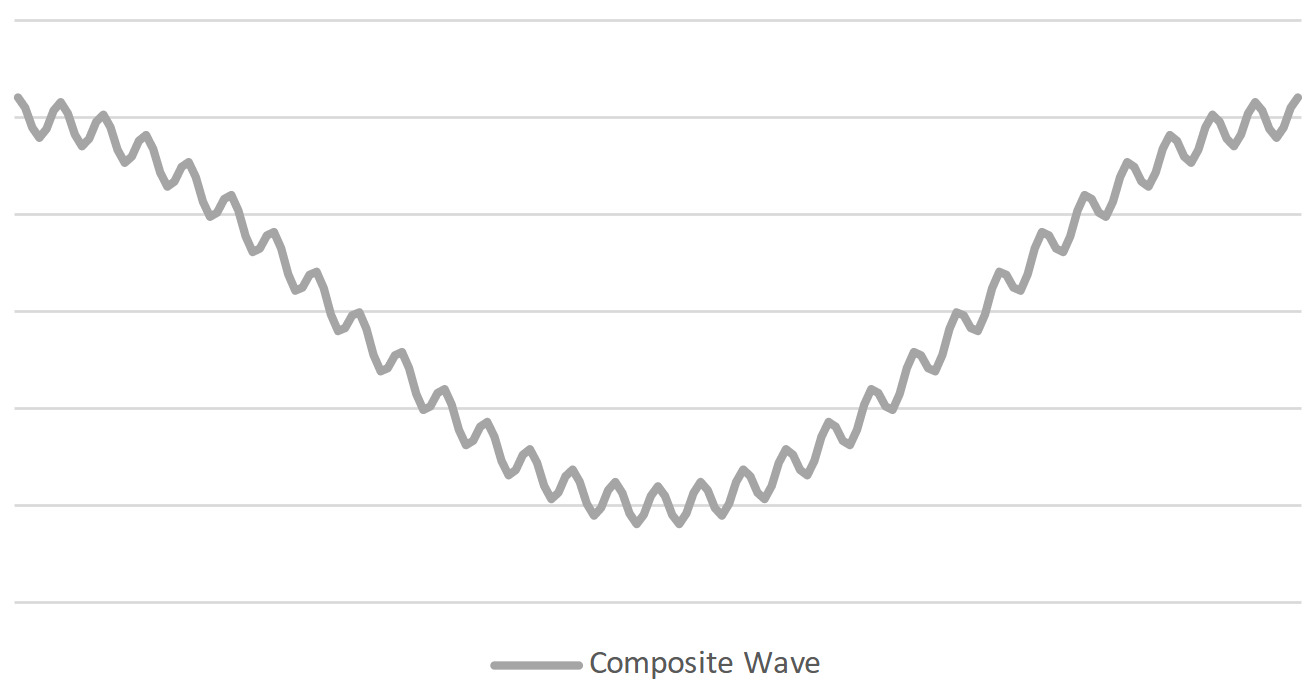
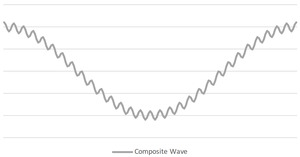
In applications using the DFT, analysts simplify their models by discarding frequencies that they consider to be noise in their data. Or more precisely, the noise frequencies comprise the error distribution. The decision criteria for inclusion in the model favors the frequencies with the largest amplitudes, and often favor low frequencies over higher frequencies. To illustrate this second point, when modeling long-term economic trends, they might discard frequencies associated with annual seasonality, even though the magnitude of the seasonal element may be significant. This selection process is illustrated in the following graphs.

The graph above depicts two harmonic functions. One has a low frequency and large amplitude, while the other has a high frequency and lower amplitude. The sum of the two harmonics is shown below. It should be clear that in most situations, analysts would choose the low-frequency long-period cycle to be the signal and consign the high frequency harmonic to the error distribution.

6. Summary and Conclusion

Equating the LaPlace transform with stochastic present value is equivalent to relaxing the present value assumptions to allow complex numbers in the exponent. The LaPlace transform accommodates both stochastic rates and stochastic amounts. The only question is whether we can visualize the transform and attach meaning to it.

If we allow a complex exponent in the present value formula, the real part of the exponent is a discount rate, while the imaginary part is a frequency. In our normal frame of reference, we model relative frequency by amount, while in the transform space we model amount by frequency.

The transform is complex valued, but the inverse recovers real valued outcomes. Pairs of complex exponentials form real valued sines and cosines. Using the LaPlace transform is similar in process to using a log transform; we transform our data, perform operations that are easier in the transform space, then transform back.

When modeling stochastic rates, we can visualize the transform to be finding waves around the exponential trend. When modeling stochastic cash flows, we visualize the DFT interpolating time series data with waves around the sample mean.

---