Unifying Triangle-Based Actuarial Reserving Method

undefined

1. Introduction

Actuarial reserving of property-casualty exposures commonly relies on triangle-based methods. The two most common methods for actuarial reserving are the chain-ladder and Bornhuetter-Ferguson (B-F) methods.

Actuaries will commonly develop projections using multiple triangle-based projection methods. These multiple methods offer competing projections of ultimate claims that the actuary will (implicitly or explicitly) weight to establish a single “selected” estimate.

In this paper, I attempt to address the following shortcomings of this approach.

Selection of ultimate claims There are no approaches in common use for the weighting of competing indications. I presented an approach in Applying Credibility Concepts to Develop Weights for Ultimate Claim Estimators. The approach in that paper requires additional analysis to implement, and I have not observed the method in use.

No direct variance measure Triangle-based methods provide point estimates. If we considered each method as an independent univariate regression model (as described later in this paper), we would have access to a variance model for that method (in isolation). The multivariate model provides the variance of the selection.

Lack of flexibility The implementation of a particular triangle-based method assume that it is an appropriate approach to project claims amounts from the current maturity to ultimate. For example, the methods don’t allow for the possibility that, for an accident year valued at 12 months, the B-F method is a better predictor of emergence between 12 and 36 months, but that the chain-ladder method is the better predictor after 36 months.

There is an important limitation to the approach I present. The model can not be used to extrapolate beyond the end of the triangle. That is, we can use the modeling approach to “square the triangle,” but not to extend of the square to an “ultimate rectangle.” Such an extension is beyond the scope of this paper and there are several approaches in the actuarial literature discussing such extensions.

1.1. Past Research

The idea of using regression models for prediction is not new. For example, “Loss Development Using Credibility” (J Eric Brosius, CAS Exam Study Note, 1993) introduces least squares regression as an approach to incorporate credibility. Other research^[1] identified by the author also refers to the use of multivariate models to combine estimators. This paper has a slightly different focus than prior work. In particular, my goals for the approach presented in this paper differ from the goals of that research. In addition, I seek to present a practical, rather than theoretical, treatment of the subject.

1.2. Organization

I intend this paper to be practical. This paper includes all R code required to reproduce the results presented. In addition, I will post the Rmarkdown files used to create this paper to a repository on the CAS Github site. The downside is that you will likely need to have a base level of R knowledge to fully understand the implementation of the ideas proposed in that paper. Although a detailed discussion of the R output is beyond the scope of the paper, I will try to provide high-level interpretations of the results. I also insert comments to describe the purpose of the code that follows. In the R code, I avoid using packages (or extensions) except where necessary.

In Section 2, I demonstrate how to express each triangle-based method as a univariate linear model. Those univariate regressions have a common response variable with different explanatory variables (i.e., predictors).

In Section 3, I propose a multivariate linear model to unify these methods.

Section 4 provides concluding remarks.

1.3. Data

The worked example in this paper uses the data from Section G of the Institute and Faculty of Actuaries Claims Reserving Manual. The scope of this paper does not include consideration of required data adjustments (e.g., Berquist-Sherman adjustments or premium on-leveling), so I assume that the data is internally consistent.

1.4. Notation

We use the naming convention from the data source with accident years, $a$, numbered, $1, \ldots, 6$ and development ages, $d$, numbered $0, \ldots, 5$.

I use $r_{a, d}$ and $p_{a, d}$ to refer to incremental reported claims and incremental paid claims, respectively, from the $a^{th}$ accident year emerging the $d^{th}$ development interval.

I use and $e_a$ to refer to exposure (e.g., expected claims, premiums, vehicle-years, payroll) for the $a^{th}$ accident year, and I use $\mathit{elr}_a$ to refer to the expected loss rate for the $a^{th}$ accident year. I use $\mathit{el}_a$ refer to the product of the exposure ($e_a$) and expected loss rate ($\mathit{elr}_a$) for the $a^{th}$ accident year.

I use $\mathit{ldf}_{a, d_0 \rightarrow d_1}$ to refer to the factors relating claim amounts at $d_1$ to claim amounts at $d_0$ for accident year $a$. This factor is analogous to the loss development factor used in the chain-ladder method. The principal difference is that because I am predicting incremental claim amounts, the factor will not include the constant (unity), representing prior period cumulative claims, included in a typical loss development factor. We will refer to the vector of $\mathit{ldf}\text{s}$ as a loss development pattern.

I use $\mathit{lef}_{a, d_0 \rightarrow d_1}$ to refer to the claims emerging between $d_0$ and $d_1$ for accident year $a$ as a percentage of exposure or expected claims. We note that actuaries do not commonly calculate this factor independently in developing B-F indications but rather use emergence factors implied by the loss development pattern from the chain-ladder method.

For both the $\mathit{ldf}$ and the $\mathit{lef}$, we initially assume the factor does not differ by accident year and exclude the first subscript. This assumption is common in practice.

1.5. R Objects

We create paid, reptd and premium objects in R with the following code:

# Premium
premium <- c(4486, 5024, 5680, 6590, 7482, 8502)

# Cumulative Paid claims
paid <- matrix(c( 1001, 1855, 2423, 2988, 3335, 3483,
    1113, 2103, 2774, 3422, 3844, NA, 
    1265, 2433, 3233, 3977, NA, NA, 
    1490, 2873, 3880, NA, NA, NA, 
    1725, 3261, NA, NA, NA, NA, 
    1889, NA, NA, NA, NA, NA), nrow = 6, byrow = TRUE)

# Name the dimensions
dimnames(paid) <- list(a = 1:6, d = 0:5)

# Convert to Incremental Triangle
paid[, c(1, 2, 3, 4, 5)] <- paid[, c(1, 2, 3, 4, 5)] - 
  paid[, c(0, 1, 2, 3, 4)]

# Cumulative Reported claims
rptd <- matrix(c(
    2777, 3264, 3452, 3594, 3719, 3717, 
    3252, 3804, 3973, 4231, 4319, NA, 
    3725, 4404, 4779, 4946, NA, NA, 
    4521, 5422, 5676, NA, NA, NA, 
    5369, 6142, NA, NA, NA, NA, 
    5818, NA, NA, NA, NA, NA), nrow = 6, byrow = TRUE)

# Name the dimensions
dimnames(rptd) <- list(a = 1:6, d = 0:5)

# Convert to Incremental Triangle
rptd[, c(1, 2, 3, 4, 5)] <- rptd[, c(1, 2, 3, 4, 5)] - 
  rptd[, c(0, 1, 2, 3, 4)]

1.6. A Minimal Working Example

Readers will observe that these triangles are “small.” That is, there are only five development observations between $d = 0$ and $d = 1$, and fewer for later intervals. Since the number of observations needs to exceed the number of predictors (i.e., methods), we are limited in the size of the multivariate models. The worked example in Section 3, uses the proposed multivariate model to predict the three unknown claims amounts at $d = 1$ and $d = 2$.

In practice, actuaries analyze significantly larger triangles. Such triangles (i.e., datasets) will allow for the use of additional predictors in the multivariate model.

2. Expressing Actuarial Methods as Linear Models

The section provides the foundation for our approach by presenting actuarial methods as linear models. We provide a discussion of the chain-ladder and B-F methods. We discuss other predictors in the final section.

2.1. Chain Ladder

We recognize the prediction of the chain-ladder method has the following form^[2]:

$$r_{6, 1} = \mathit{ldf}_{0 \rightarrow 1} \times r_{6, 0}\\ $$

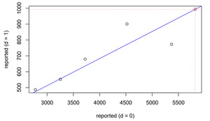
In the chain ladder method, actuaries develop estimators for $ldf_{0 \rightarrow 1}$. We should recognize this as an equation in the form $y = mx$ using “slope-intercept” notation. With that recognition, we understand that we can estimate $ldf_{0 \rightarrow 1}$ by fitting the following linear model (without an constant term) to the observed data (i.e., $r_{1\ldots5, 0\ldots1}$):

r_0 <- rptd[1:5, '0']  # The predictor; claims at age = 0
r_1 <- rptd[1:5, '1'] # The response; claims at age = 1

# Fit a linear model relating the response to the predictor
# The + 0 instructs r to not include an intercept/constant
cl_0_1 <- lm(r_1 ~ r_0 + 0)

# Print a summary of the linear model
summary(cl_0_1)

## 
## Call:
## lm(formula = r_1 ~ r_0 + 0)
## 
## Residuals:
##       1       2       3       4       5 
##   12.95   -3.14   43.12  129.23 -143.53 
## 
## Coefficients:
##     Estimate Std. Error t value Pr(>|t|)    
## r_0  0.17071    0.01099   15.53    1e-04 ***
## ---
## Signif. codes:  0 '***' 0.001 '**' 0.01 '*' 0.05 '.' 0.1 ' ' 1
## 
## Residual standard error: 99.17 on 4 degrees of freedom
## Multiple R-squared:  0.9837, Adjusted R-squared:  0.9796 
## F-statistic: 241.3 on 1 and 4 DF,  p-value: 0.0001003


coef(cl_0_1)

##       r_0 
## 0.1707073

The summary function in the code block provides the results in the output above. Recall that the reptd object represents incremental values and, as a result, the fitted coefficient is analogous to the traditional development factor minus 1. The output indicates that the estimator coefficient is 0.17071 and the implied development factor is 1.17071.

This approach also provides metrics to support the evaluation of predictive value. We also observe the p-value (which R labels Pr(>t)) is $10^{-4}$ demonstrating statistical significance at the commonly used 5% threshold. We also observe that the model explains a significant portion of the variability (i.e., the adjusted R-squared is high at 0.98).

The fitted coefficient, $\hat{b}_{\mathit{CL}, 0 \rightarrow 1}$, is an estimator for $ldf_{0 \rightarrow 1}$ and we can use that estimator to predict $r_{6, 1}$.

$$\hat{r}_{6, 1} = \hat{b}_{\mathit{CL}, 0 \rightarrow 1} \times r_{6, 0} + \epsilon$$

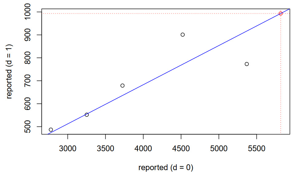
We can observe the relationship visually in the following figure.

# Predicted value for r(6,1)
c_1 <- predict(object = cl_0_1, newdata = data.frame(r_0 = rptd['6', '0']))

# Review the linear model visually
plot(x = rptd[1:6, 0], y = c(r_1, c_1), col = c(rep('black', 5), 'red'), 
    main = 'Chain-Ladder', xlab = 'reported (d = 0)', 
    ylab = 'reported (d = 1)') 
abline(cl_0_1, col = 'blue') # Plot the fitted model

# The prediction (in red)
abline(v = rptd['6', '0'], lty = 'dotted', col = 'red') 
abline(h = c_1, lty = 'dotted', col = 'red')

2.2. Bornhuetter-Ferguson

Using the same principles, we recognize the prediction of the B-F method has the following form:

$$r_{6, 1} = \mathit{lef}_{0 \rightarrow 1} \times \mathit{elr}_{6} \times e_{6}$$ As noted, we assume that exposure is internally consistent and doesn’t require an adjustment for exposure trend or on-leveling for rate changes.

In the B-F method, actuaries require an estimator for $\mathit{lef}_{0 \rightarrow 1}$. In practice actuaries use the results of the chain-ladder modeling for this estimator.

We again recognize that this form is analogous to a linear model without an intercept term. In this model, $\mathit{elr}_{.} \times e_{.}$ is the predictor. Critically for the concepts described in this paper, the response variable is the same as the response variable in the linear model for the chain-ladder method.

Assuming that the expected loss ratio is constant but unknown, we could express the equivalent univariate regression as follows.

$$\hat{r_{6, 1}} = \hat{b}_{\mathit{BF}, 0 \rightarrow 1} \times e_{6}$$ In this case, our predictor is the product of the expected claims ratio, $\mathit{elr}$, and the $\mathit{lef}$. We will use this approach for generality.

If we had a working assumption for the expected claims, then our independent variable would be the product of $\mathit{elr}_{.}$ and $e_{.}$ ,i.e., $el_{.}$, and we would express our prediction as follows.

$$\hat{r}_{6, 1} = \hat{b}_{\mathit{BF}, 0 \rightarrow 1} \times el_{6}$$

In this case, our estimated regression coefficient would be the estimator of $\mathit{lef}_{\mathit{BF}, 0 \rightarrow 1}$. As with the chain-ladder discussion in the prior section, note that the we are predicting incremental values, so we do not include the “to-date” claim amounts included as an additive term in the B-F formula.

e <- premium[1:5] # predictor
r_1 <- rptd[1:5, '1'] # response

# Fit the linear model "through the origin"
bf_0_1 <- lm(r_1 ~ e + 0)

# Print a model summary
summary(bf_0_1)

## 
## Call:
## lm(formula = r_1 ~ e + 0)
## 
## Residuals:
##      1      2      3      4      5 
## -33.37 -30.78  20.13 136.57 -94.90 
## 
## Coefficients:
##   Estimate Std. Error t value Pr(>|t|)    
## e 0.115998   0.006522   17.79 5.87e-05 ***
## ---
## Signif. codes:  0 '***' 0.001 '**' 0.01 '*' 0.05 '.' 0.1 ' ' 1
## 
## Residual standard error: 86.78 on 4 degrees of freedom
## Multiple R-squared:  0.9875, Adjusted R-squared:  0.9844 
## F-statistic: 316.3 on 1 and 4 DF,  p-value: 5.872e-05

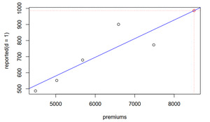
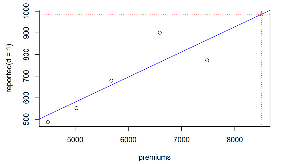
As with the chain-ladder model, we note that the coefficient is statistically significant $p =$ $5.872\times 10^{-5}$ and the model explains a significant portion of the variability (adjusted R-squared =0.984).

c_1 <- predict(object = bf_0_1, newdata = data.frame('e' = premium[6])) 
plot(x = premium, y = c(r_1, c_1), col = c(rep('black', 5), 'red'), 
    main = 'Bornhuetter-Ferguson', xlab = 'premiums', ylab = 'reported(d = 1)') 
abline(bf_0_1, col = 'blue')

# The prediction
abline(v = premium[6], lty = 'dotted', col = 'red') 
abline(h = c_1, lty = 'dotted', col = 'red')

2.3. New Insight

Using this approach we no longer need to rely on the anecdotal advantages of stability and responsiveness associated with B-F and chain ladder, respectively. More accurately, the notion that we should use B-F for immature claim cohorts and chain ladder for mature cohorts is no longer necessary as, under the approach presented in this paper, we receive statistical feedback as to the predictive value of each method.

2.4. Additional Predictors

We can use this concept to expand to other candidate predictors. We provide a discussion of two such candidates below.

Paid claims It is reasonable to assume that future claim reporting may be a function of prior claim payments. In a spreadsheet, the actuary would construct a triangle of ratios of incremental reported claims to prior cumulative paid claims and apply a chain-ladder model to that triangle.

Case reserves We should recognize that (particularly for classes of business with fast claims reporting), case reserves are often considered predictive for future claims reporting. For this reason, actuaries often assess the reasonableness of estimates using IBNR to case ratios.

As we add predictors, we should recognize that reported claims are a linear combinations of paid claims and case reserves. As such, we can only use any two of these three metrics in the multivariate model that we introduce in the next section.

Idiopathic additive We should also appreciate that the reported claim amounts may be idiopathic. That is, they may not be proportional to any specific predictors. In regression, we refer to this idiopathic estimate as the “constant” or “intercept”.

It is beyond the scope of this paper to list all potential predictors. Rather, it is our goal to introduce the expression of models as univariate regressions. The actuary should recognize several other potential predictors, such as open claim counts or the prior evaluation of ultimate claims. That is the thesis of this research: Once we appreciate that we can express triangle-based methods as linear models, the possibilities become limitless.

3. The Multivariate Model

In this section, we will present the prediction of reported claim values in the multivariate model. We demonstrate the approach by first predicting the reported claim value at $(a = 6, d = 1)$: $r_{6, 1}$ using reported development and reported B-F approaches. As a demonstration of the model’s flexibility, we then consider approaches that actuaries generally do not consider. That is, we predict incremental reported amounts that are idiopathic and predict incremental reported amounts with paid claim amounts as a predictor. That is, in addition to the idiopathic potential, we have three candidate predictors: reported claims, paid claims and exposures.

An identical approach can also be (and should also be) used to predict paid claim values.

3.1. The Saturated Model

We can develop and fit a model using all of our candidate predictors. We refer to this as our saturated model. Below we present two saturated models. The first includes an intercept; the second does not^[3].

r_1 <- rptd[1:5, '1'] # Response

r_0 <- rptd[1:5, '0'] # Predictor
p_0 <- paid[1:5, '0'] # Predictor
e <- premium[1:5] # Predictor

# Saturate model with intercept
full_lm <- lm(r_1 ~ r_0 + p_0 + e) 
summary(full_lm)

## 
## Call:
## lm(formula = r_1 ~ r_0 + p_0 + e)
## 
## Residuals:
##       1       2       3       4       5 
##   9.853   9.281 -66.038  74.741 -27.836 
## 
## Coefficients:
##              Estimate Std. Error t value Pr(>|t|)
## (Intercept) -1550.193   1481.136  -1.047    0.485
## r_0            -1.314      1.753  -0.750    0.591
## p_0            -1.110      6.842  -0.162    0.898
## e               1.513      1.129   1.340    0.408
## 
## Residual standard error: 104.4 on 1 degrees of freedom
## Multiple R-squared:  0.9019, Adjusted R-squared:  0.6074 
## F-statistic: 3.063 on 3 and 1 DF,  p-value: 0.3923


# Saturate model without intercept (i.e., "through the origin")
full_lm_origin <- lm(r_1 ~ r_0 + p_0 + e + 0) 
summary(full_lm_origin)

## 
## Call:
## lm(formula = r_1 ~ r_0 + p_0 + e + 0)
## 
## Residuals:
##      1      2      3      4      5 
##  13.97 -72.60 -15.41 119.62 -53.29 
## 
## Coefficients:
##     Estimate Std. Error t value Pr(>|t|)
## r_0   0.4027     0.6331   0.636    0.590
## p_0  -4.6798     6.0713  -0.771    0.521
## e     0.9004     0.9878   0.912    0.458
## 
## Residual standard error: 106.9 on 2 degrees of freedom
## Multiple R-squared:  0.9905, Adjusted R-squared:  0.9763 
## F-statistic: 69.71 on 3 and 2 DF,  p-value: 0.01418

Interestingly we note the following:

• The model with the intercept has a lower adjusted R-squared than the model without the intercept. In addition, the signs of the coefficients of the model with the intercept are not intuitive. These observations are not surprising, as we should have noted the increasing volumes when examining the data. With that increasing volume, it would be surprising if the intercept (idiopathic) term added predictive value.

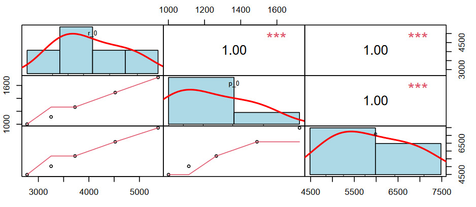
• Although the model without the intercept predicts a significant portion of the variability, none of the predictors is statically significant. This observation is also not terribly surprising since, as with any linear model, the actuary needs to be concerned with the collinearity of predictors. We present a test of that collinearity below.

The following code produces a chart to support the analysis of correlations. The charts on the diagonal present distributions of each predictor variable. The charts on the lower left present scatter plots; the upper right blocks present pearson correlation coefficients.

corr_chart(data.frame('r_0' = r_0, 'p_0' = p_0,
    'e' = e), cex = 0.7, cex.labels = 0.7)

With the high correlations, we need not proceed further with additional testing. For example, if the correlations were lower, we could use an F-test to compare saturated and reduced models. We recognize that we do not need to use multiple predictors (methods) with this particular dataset. In the next section, we discuss how to proceed to model selection given the results of our testing.

3.2. Model Selection

Although perhaps not in a wholly satisfying way, this brings us to an inflection point in our journey to predict $r_{6,1}$ with the following conclusions:

• There is no idiopathic development in this triangle due to increasing volumes.

• Paid claims, reported claims and exposures are highly correlated. As a result, adding predictors (i.e., additional methods) does not add significant incremental value.

However, the same conditions would apply to a traditional approach - very consistent predictions across methods. Potentially there would be differences between B-F and chain ladder since the loss emergence factors are not calibrated to the predictor. We should appreciate that this approach provides the actuary with an understanding of the basis for that consistency.

We present the summaries of the univariate models^[4].

# B-F
lm(r_1 ~ e + 0) |> summary ()

## 
## Call:
## lm(formula = r_1 ~ e + 0)
## 
## Residuals:
##      1      2      3      4      5 
## -33.37 -30.78  20.13 136.57 -94.90 
## 
## Coefficients:
##   Estimate Std. Error t value Pr(>|t|)    
## e 0.115998   0.006522   17.79 5.87e-05 ***
## ---
## Signif. codes:  0 '***' 0.001 '**' 0.01 '*' 0.05 '.' 0.1 ' ' 1
## 
## Residual standard error: 86.78 on 4 degrees of freedom
## Multiple R-squared:  0.9875, Adjusted R-squared:  0.9844 
## F-statistic: 316.3 on 1 and 4 DF,  p-value: 5.872e-05

# C- L
lm(r_1 ~ r_0 + 0) |> summary ()

## 
## Call:
## lm(formula = r_1 ~ r_0 + 0)
## 
## Residuals:
##       1       2       3       4       5 
##   12.95   -3.14   43.12  129.23 -143.53 
## 
## Coefficients:
##     Estimate Std. Error t value Pr(>|t|)    
## r_0  0.17071    0.01099   15.53    1e-04 ***
## ---
## Signif. codes:  0 '***' 0.001 '**' 0.01 '*' 0.05 '.' 0.1 ' ' 1
## 
## Residual standard error: 99.17 on 4 degrees of freedom
## Multiple R-squared:  0.9837, Adjusted R-squared:  0.9796 
## F-statistic: 241.3 on 1 and 4 DF,  p-value: 0.0001003


# Reported ~ Paid
lm(r_1 ~ p_0 + 0) |> summary ()

## 
## Call:
## lm(formula = r_1 ~ p_0 + 0)
## 
## Residuals:
##       1       2       3       4       5 
##  -26.61  -19.08   29.93  136.49 -112.09 
## 
## Coefficients:
##     Estimate Std. Error t value Pr(>|t|)    
## p_0  0.51310    0.03029   16.94 7.12e-05 ***
## ---
## Signif. codes:  0 '***' 0.001 '**' 0.01 '*' 0.05 '.' 0.1 ' ' 1
## 
## Residual standard error: 91.05 on 4 degrees of freedom
## Multiple R-squared:  0.9863, Adjusted R-squared:  0.9828 
## F-statistic:   287 on 1 and 4 DF,  p-value: 7.119e-05

The predictive quality of the models is essentially equivalent. We’d consider all of the models to be reasonable. The B-F model is very marginally better than the others, so we select that model for our prediction of $r_{6,1}$. As noted, a benefit of our approach is that regression output includes (frequentist) measures of standard errors. We now use that property to develop the distribution of $r_{6,1}$.

3.3. Reported Claim Prediction

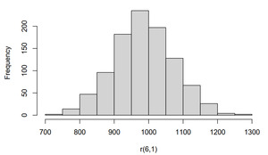
Now we can use our selected model for prediction. Importantly, the use of linear models allows for the modeling of variability. We present the (simulated) the distribution of $r_{6,1}$ below.

# Mean and standard deviation of the predictors
mean_r_6_1 <- predict(object = bf_0_1, newdata = data.frame('e' = premium[6]))
sd_r_6_1 <- summary(bf_0_1)$sigma

# linear models assume normality
# pipe the result to the hist function to present the distribution
r_6_1 <- rnorm(n = 1e3, mean = mean_r_6_1, sd = sd_r_6_1) |>
hist(xlab = 'r(6,1)', main = 'Histogram of Predictions')

We now have a model for r(6,1) which:

• Considers the predictive value of multiple predictors.

• Directly provides a measure of variability.

3.4. Paid Claim Prediction

For brevity, we do not provide the details of the paid claim prediction. However, since we are aware of the high correlation of the predictors, we can advance directly to a review of the prediction of paid claims.

p_1 <- paid[1:5, '1'] 
# B-F
lm(p_1 ~ e + 0) |> summary ()

## 
## Call:
## lm(formula = p_1 ~ e + 0)
## 
## Residuals:
##      1      2      3      4      5 
## -59.37 -32.91  11.52  41.24  12.63 
## 
## Coefficients:
##   Estimate Std. Error t value Pr(>|t|)    
## e 0.203605   0.003053   66.69 3.03e-07 ***
## ---
## Signif. codes:  0 '***' 0.001 '**' 0.01 '*' 0.05 '.' 0.1 ' ' 1
## 
## Residual standard error: 40.62 on 4 degrees of freedom
## Multiple R-squared:  0.9991, Adjusted R-squared:  0.9989 
## F-statistic:  4447 on 1 and 4 DF,  p-value: 3.03e-07


# C- L
lm(p_1 ~ p_0 + 0) |> summary ()

## 
## Call:
## lm(formula = p_1 ~ p_0 + 0)
## 
## Residuals:
##      1      2      3      4      5 
## -48.17 -13.11  27.89  40.11 -18.69 
## 
## Coefficients:
##     Estimate Std. Error t value Pr(>|t|)    
## p_0  0.90127    0.01203   74.94  1.9e-07 ***
## ---
## Signif. codes:  0 '***' 0.001 '**' 0.01 '*' 0.05 '.' 0.1 ' ' 1
## 
## Residual standard error: 36.15 on 4 degrees of freedom
## Multiple R-squared:  0.9993, Adjusted R-squared:  0.9991 
## F-statistic:  5616 on 1 and 4 DF,  p-value: 1.9e-07


# Paid ~ Reported
lm(p_1 ~ r_0 + 0) |> summary ()

## 
## Call:
## lm(formula = p_1 ~ r_0 + 0)
## 
## Residuals:
##      1      2      3      4      5 
##  20.47  13.90  49.92  26.00 -75.53 
## 
## Coefficients:
##     Estimate Std. Error t value Pr(>|t|)    
## r_0 0.300155   0.005396   55.62 6.26e-07 ***
## ---
## Signif. codes:  0 '***' 0.001 '**' 0.01 '*' 0.05 '.' 0.1 ' ' 1
## 
## Residual standard error: 48.7 on 4 degrees of freedom
## Multiple R-squared:  0.9987, Adjusted R-squared:  0.9984 
## F-statistic:  3094 on 1 and 4 DF,  p-value: 6.256e-07

Again, we note that all three models are highly predictive. We select the paid chain ladder model as it has the highest R-squared value.

pcl_0_1 <- lm(p_1 ~ p_0 + 0)

mean_p_6_1 <- predict(object = pcl_0_1, 
    newdata = data.frame('p_0' = paid[6, '0']))
sd_p_6_1 <- summary(pcl_0_1)$sigma
p_6_1 <- rnorm(n = 1e3, mean = mean_p_6_1, sd = sd_p_6_1) |>
    hist(xlab = 'p(6,1)', 
    main = 'Histogram of Incremental Paid Claim Predictions')

3.5. The Next Interval

We now turn to predictions of reported and paid claim values at $(a = 5, d = 2)$ and at $(a = 6, d = 2)$. For brevity, we don’t repeat the discussion above. However, we should recognize that these predictions will differ from the prediction of $(a = 6, d = 1)$ in important ways.

• We have added predictors. That is, we can predict $r_{(6,2)}$ using either cumulative reported $\sum_{i = 0}^{1} r_{6, i}$, or incremental ($r_{(6,0)}$ or $r_{(6,1)}$) reported. We should bear in mind that we can not use $r_{(6,1)}$, $r_{(6,2)}$, and $\sum_{i = 0}^{1} r_{6, i}$ as the cumulative amount is a linear combination of the two incremental values.

• Our predictions of $r_{(6,2)}$ consider our prediction of $r_{(6,1)}$. That is, the output of the prior step becomes data in this step.

• We now have many more potential predictors than data points. Therefore, testing alternatives against a saturated model with all predictors is not an option. However, if we can eliminate a few predictors in a first step, then we may still be able to pursue this approach.

Below, we present sample R code to support the evaluation of alternative predictors. The R object pred_list is a list of potential predictors. In order, those predictors are reported claims in emergence interval 0, reported claims in emergence interval 1, exposures, cumulative reported claims at the end of interval 1, paid claims in emergence interval 0, paid claims in emergence interval 1, and cumulative paid claims at the end of interval 1. We then instruct R to return the $R^2$ value for each model and coefficient information including p- values. The lapply function is the R version of a loop as it applies the function to each predictor. The function that I defined prints the adjusted R-squared value and the model coefficients.

r_2 <- rptd[1:4, '2']

pred_list <- list('r_0' = rptd[1:4, '0'], 
    'r_1' = rptd[1:4, '1'], 'e' = e[1:4],
    'r_tot' = rptd[1:4, '0'] + rptd[1:4, '1'], 'p_0' = paid[1:4, '0'],
    'p_1' = paid[1:4, '1'], 'p_tot' = paid[1:4, '0'] + paid[1:4, '1'])
    
lapply(X = names(pred_list), FUN = function(predictor){
    pred <- pred_list[[predictor]]
    print(predictor)
    paste('adjusted r-squared =', summary(lm(r_2 ~ pred + 
        0))$adj.r.squared |> round(4)) |> print()
    
      summary(lm(r_2 ~ pred + 0))$coefficients |> print()
}) |> invisible()

## [1] "r_0"
## [1] "adjusted r-squared = 0.8991"
##        Estimate Std. Error  t value    Pr(>|t|)
## pred 0.06875884 0.01135696 6.054336 0.009040266
## [1] "r_1"
## [1] "adjusted r-squared = 0.8864"
##       Estimate Std. Error  t value   Pr(>|t|)
## pred 0.3682799  0.0648792 5.676394 0.01083279
## [1] "e"
## [1] "adjusted r-squared = 0.9034"
##        Estimate  Std. Error  t value    Pr(>|t|)
## pred 0.04540309 0.007327219 6.196498 0.008467226
## [1] "r_tot"
## [1] "adjusted r-squared = 0.8978"
##        Estimate  Std. Error  t value    Pr(>|t|)
## pred 0.05797275 0.009643283 6.011724 0.009221901
## [1] "p_0"
## [1] "adjusted r-squared = 0.9019"
##       Estimate Std. Error  t value    Pr(>|t|)
## pred 0.2027884 0.03299423 6.146179 0.008664453
## [1] "p_1"
## [1] "adjusted r-squared = 0.907"
##       Estimate Std. Error  t value    Pr(>|t|)
## pred 0.2240414 0.03541276 6.326571 0.007984001
## [1] "p_tot"
## [1] "adjusted r-squared = 0.9046"
##       Estimate Std. Error  t value    Pr(>|t|)
## pred 0.1064681 0.01706105 6.240419 0.008299867

Based on this review, we may elect to use a predictor for $r_{(6,2)}$ that is different than we used for $r_{(6,1)}$. We now recognize the flexibility advantage of the approach in this step. For example, we note that the highest $R^2$ value is for the model that uses paid amounts in interval 1 (a type of chain-ladder model) as the predictor. We have a triangle-based model that considers B-F and chain ladder, but this model recognizes that different predictors methods may be optimal in different intervals.

3.6. Uncertainty Modeling

As noted, we now have a model for our response variable. That is, we can simulate each of the response variables using the fitted model. If we create a decision rule (e.g., “Use the model with the highest adjusted $R^2$.”) we can write code to generate the entire lower half of the triangle. The recipe would the code would be as follows.

1. Fit candidate models to estimate $r_{(6,1)}$.

2. Use a decision rule to select from the candidate models.

3. Simulate a value for $r_{(6,1)}$.

4. Using that simulated value and the data repeat the process for $r_{(5,2)}$ and $r_{(6,2)}$

5. Repeat to “square the triangle”

3.7. The Last Interval

When we reach the last column of data, we could be in one of two positions: (i) the data could be judged to be at (or close to) ultimate, or (ii) there could be development beyond the triangle.

In our example, we are not yet at ultimate as we observe that reported and paid claims are not equal at $(a = 1, d = 5)$. In this case, we can apply the algorithm described above separately to paid and reported claims. Then we must use approaches beyond the scope of this paper to extend predictions to ultimate.

However, if we had observed that the data were at ultimate at an age within the triangle, then we would not want to estimate both paid and reported claims at that age, as they would be equal. We would fit linear models to the observed ultimate claims (equal to observed paid or reported claims, which would be equal) using whatever predictors we have at our disposal.

4. The Final Word

In this paper I demonstrate that triangle-based methods can be expressed as univariate models. This approach offers several improvements relative to current practice.

Additional Predictors Triangle-based methods are linear models with different predictors. That is, we can effectively use “predictors” and “method” interchangeably. This recognition then opens the universe of potential predictors (methods).

Statistical Basis to Combine Estimates We can then combine the predictors using a multivariate model, which provides a statistical basis to combine the results of various methods rather than judgmental selection.

Uncertainty Models Linear models naturally provide uncertainty information. The approach will directly provide the distribution of outcomes.

Flexibility The combination of methods doesn’t occur in the final selection of ultimate but also to the predictions at earlier ages. As such, this approach recognizes that different methods may be better predictors of incremental claims within the triangle. Current approaches assume that the same predictor is optimal at all ages.

Unfortunately, the publicly-available example data in this paper did not offer the most interesting implementation of this model. Please contact the author if you have an example dataset that would provide an opportunity to further this research.

---

Acknowledgement

I thank Ryan Royce and Francis (Frank) Costanzo for their thoughtful and timely reviews of drafts of this paper. I also thank them for their patience. Any errors that remain in this paper are the responsibility of the author.

---

1. for example, “Combining Chain-Ladder and Additive Loss Reserving Methods for Dependent Lines of Business”, Michael Merz and Mario V. Wüthrich, Variance, 2009, and “Optimal and Additive Loss Reserving for Dependent Lines of Business”, Klaus D. Schmidt, Casualty Actuarial Society E-Forum, Fall 2006.

2. I recognize this form lack generality. That is, estimates for later ages require the sum of reported values for all prior ages which is not included in this presentation.

3. The + 0 at the end of the specification for full_lm_origin instructs R to fit a model without a constant/intercept, i.e. “through the origin.”

4. Note we use the R native pipe operator >. With the pipe operator a > function() is the same as function(a).