Alternative to Tweedie in Pure Premium GLM

undefined

1. INTRODUCTION

“Statisticians, like artists, have the bad habit of falling in love with their models.”
—George E. P. Box

The introduction of Generalized Linear Models (GLM) in ratemaking in the 1990’s was a great step for Actuarial techniques and brought greater computational efficiency and flexibility to ratemaking. Extensions for mixed models (GLMM), generalized estimating equations (GEE) and additive models (GAM) have expanded the usefulness of the technique even further.

However, one assumption made early on has never really been challenged. The general approach is that a Tweedie variance structure is recommended for pure premium (i.e., aggregate loss rather than separate frequency and severity models). The main argument seems to have been that the Tweedie, when constraining the variance parameter 1<p<2 can be interpreted as a collective risk model with Poisson frequency and Gamma severity.

True enough.

But there is a rival to the Tweedie variance structure that also has a collective risk model interpretation: the quasi-negative binomial (QNB). The QNB can be interpreted as a Poisson frequency with a [discretized] logarithmic severity. The logarithmic distribution is derived by mixing the mean parameter of a geometric random variable using an upper-truncated Pareto as the mixing distribution; it can be viewed as a discrete version of a mixed exponential model for severity.

Like the Tweedie, the QNB is a three-parameter curve that behaves like a compromise between the Poisson and Gamma variance structures. The difference between them is only in the behavior of the variance function. And the QNB follows the assumptions of collective risk loss models more closely.

For more details on the Negative Binomial, including code, interested readers are referred to the book-length treatment by Hilbe.

2. VARIANCE OF COLLECTIVE RISK MODELS

In a traditional collective risk model, we have a random variable N representing frequency, and a random variable X representing severity. The aggregate loss Z is the sum of N independent draws from the severity distribution.

$$Z=\sum_{j=1}^{N} X_{j} \tag{2.1}$$

The variance of the aggregate loss distribution is given by:

$$\begin{align} Var(Z)&=Var(X) \cdot E(N)\\ &\quad +E(X)^{2} \cdot Var(N) \end{align} \tag{2.2}$$

If we further assume that the frequency is negative binomial, then the variance of Z can be written as the sum of two components: first a multiple of the expected loss, second a multiple of expected loss squared.

$$Var(N)=E(N)+c \cdot E(N)^{2} \tag{2.3}$$

$$\begin{align} Var(Z)&=\left(\frac{E\left(X^{2}\right)}{E(X)}\right) \cdot E(Z)\\ &\quad +c \cdot E(Z)^{2} \end{align} \tag{2.4}$$

This structure can also be interpreted as a process variance component plus a non-diversifiable risk component. That is, the coefficient of variation (CV) will asymptotically approach some finite percent rather than going to zero as the portfolio gets very large.

The Tweedie distribution does not share this behavior. Its variance function is defined as:

$$Var(Z)=\varnothing \cdot E(Z)^{p} \tag{2.5}$$

In this form, the dispersion parameter ϕ is estimated in the GLM but is considered a “nuisance parameter” because it does not affect the estimate of the expected loss. For the Tweedie, it is more difficult to validate the GLM results against other collective risk model work.

The QNB also includes a dispersion parameter ϕ estimated by the model. But the variance function more closely mimics the collective risk model used in other applications. The parameters ϕ and k are both in the same units as the response variable of the model.

$$\begin{align} Var(Z)&=\varnothing \cdot\biggl(E(Z)\\ &\quad +\frac{1}{k} \cdot E(Z)^{2}\biggr) \end{align} \tag{2.6}$$

3. COMPARISON OF TWEEDIE AND QNB

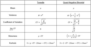
As mentioned above, both the Tweedie and the QNB can be interpreted as collective risk models and as compromises between the variance structures of Poisson and Gamma. The table below compares some of the differences in moments, especially as they change with the expected value μ.

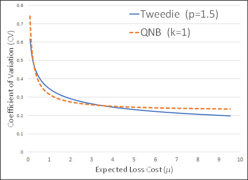
If the loss cost is similar across all classes in the rating plan, then these alternative structures will give virtually identical results. However, the variance structure for Tweedie will tend to fit better for the larger loss cost classes. This is mainly because the CV decreases faster for the Tweedie than for the QNB. Secondarily, if the Tweedie shape parameter is constrained as 1<p<2, then it will have slightly lower kurtosis, leading to more reaction to observations in the “tail” of the distribution.

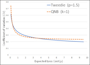
The behavior of the CV can be illustrated graphically to show that the CV is generally higher at the ends of the range of expected loss costs. The results being less sensitivity to the extremes.

If we extend the curves further to the right, the Tweedie will approach a CV of zero whereas the QNB would approach a finite number greater than zero.

4. CONCLUSIONS

The selection of a variance structure in a GLM model will not materially change the fitted values in most cases. However, what will change is the significance measures (t-statistics, p-values, etc.) used to evaluate the model parameters. Changing the variance structure could change how we view the importance of different rating variables, or even the choice of which rating variables should be included.

All of this suggests investigating use of the QNB as an alternative to the Tweedie when modeling pure premium in GLM.

---

Abbreviations and notations

CV, coefficient of variation (standard deviation divided by mean) GLM, Generalized Linear Model

QNB, Quasi-Negative Binomial (Negative Binomial with dispersion parameter to rescale)

Biography of the Author

Dave Clark is a senior actuary with Munich Reinsurance America, working with Corporate Risk and Underwriting. He is best known within the actuarial community for his study note on “Basics of Reinsurance Pricing” on the CAS examination syllabus.

He can be contacted by email at: dclark@munichre.com