


Insurance policies and reinsurance treaties can produce claims and sometimes other expenses or receipts that are affected by foreign exchange risk. The extent of risk this poses to the enterprise depends on the distribution of such exchange rate fluctuations as well as various policy features, onward reinsurance, and any other measures that are taken to hedge the risk. Regulatory models of exchange rate risk are usually quite simplistic. They are obviously important to follow but can misrepresent the true risk, and it is important for enterprise risk management (ERM) to model the risk more accurately.
This paper is divided as follows. Section 1 gives simple examples of applied exchange rate risk modeling, including regulatory models, and describes some important considerations for their use. Section 2 explains the standard economic and financial theory of exchange rate movements and volatility. Section 3 explains how various data can be used to produce exchange rate projections and confidence intervals, using the standard theory. Section 4 summarizes the main conclusions.
One might ask whether all this matters because, in the form of currency options, futures and forward contracts, and delta hedging strategies, financial markets offer a wide range of tools to hedge currency risk.[1] The answer is that hedging currency risk is generally impractical for property and casualty insurers. Measuring, limiting, and pricing of risk are the major methods by which property and casualty insurers should manage currency risk. First, implementing derivatives-based strategies to manage risk is logistically difficult, and for an organization that does not already have the capacity to do this, building such capacity would be expensive. Second, even for property and casualty insurers with the technical capacity to hedge, the transaction costs involved in doing so are prohibitive. Most examples of currency risk in property and casualty insurance involve very uncertain payment obligations. In a typical application where an insurer incurs a foreign loss liability, for example, the mean and the ninth decile of the distribution of loss in the foreign currency could vary by an order of magnitude. How much should such an insurer hedge? The reality is that financial products are not free. Standard financial market product pricing is consistent with the techniques explained here but includes margins for profit and transaction costs. Actively trading such products, to hedge enough risk to meet typical ERM Value-at-Risk (VaR) standards, for example, would be prohibitively expensive.
1. Practical examples
Foreign exchange risk can take various forms, but the greatest is typically the risk, usually called market risk, that the value of assets or liabilities denominated in a particular currency will be adversely affected by fluctuations in its exchange value into other currencies. This section introduces some models of particular kinds of market risk. The potential scope of applications extends well beyond what is described here, but I hope this section also will serve as a guide for applications that go beyond these models.
Consider a nonmarketable German €1,000,000 two-year zero-coupon note held by a US insurer. Even if the note is almost “risk-free” in the sense that there is negligible risk of default, there is a risk that the dollar value of the €1,000,000 payment at maturity will fall due to an increase in the exchange rate. What is the appropriate capital needed to support the market risk on this obligation at a 99.5% VaR level? Assume the projected future euro (EUR)/US dollar (USD) exchange rate is modeled in accordance with the theory of interest rate parity as described in Sections 2 and 3 and Appendix A.[2] Assume the current EUR/USD exchange rate is 1.121, monthly volatilty is 0.0262, and the two-year, risk-free, zero-coupon rate is 3.37% for USD assets and 1.79% for EUR assets. Substituting into Equation 8 gives us
XUSD,EUR,24∼Lognormal(0.13679,0.12835).
This gives Downside risk in this case is the risk that USD strengthens against EUR, so we care about the left tail of the distribution. Inverting the cumulative density function of gives us So the insurer’s risk at a VaR 99.5 level is that the USD value of its asset will be less than expected by
$(1.15607−0.8238)1,000,000=$332,270.
This is a future value, which we may discount to present value using the two-year USD risk-free interest rate, 3.37%, giving a present value of $310,958. This is obviously a considerable amount in relation to the note’s expected value.
Next, consider an insurance policy sold in Europe by a US insurer for a fixed premium of €1,000,000 payable immediately; with nonloss expenses of €200,000, also payable immediately; and with expected loss of €800,000, which is expected to be paid in equal parts at the end of each of the first four years after the policy is sold. There are always operational considerations, for the insurer must have appropriate accounts and professional support to handle foreign currency exchange, but assuming the premium is paid when due and immediately converted from EUR to USD net of initial expense, there will be only trivial exchange risk in the initial transactions. In this case, the market risk that stems from assets and corresponding liabilities being denominated in different currencies over time should affect only the expected loss payments. Assume the current EUR/USD exchange rate is 1.121 and projected future exchange rates are modeled in accord with the theory of interest rate parity. What is the appropriate capital needed to support the market risk on this obligation at a 99.5% VaR level? Assuming the severity distribution expressed in EUR does not change with the exchange rate EUR/USD, and that the €800,000 net receipt after payment of nonloss expense is immediately converted to USD, we can apply the methods that underlie Figure A.4. Table 1 shows a selection of data from Table A.1, with weights for each year given as the EUR payments discounted at the appropriate USD rate.
The random variable we need can be written as where each of the (for short) has a lognormal distribution. The values are not independent, because each value is correlated with the values that went before it. Appendix A describes methods for approximating the distribution of a sum of lognormal variables. For the Fenton-Wilkinson approximation we need which is straightforward, and which we can obtain using Equation 14 (the individual terms are tiresome to write out but easy to calculate in a spreadsheet). Thus we obtain
E[4∑t=1wtXt]=856,289
and
var[4∑t=1wtXt]=11,436,904,351.
Substituting these values as and into Equations 15 and 16 gives us the Fenton-Wilkinson approximation:
Lognormal(13.6526,0.1244).
To produce a simulation of the sum, we first need to simulate the sequence which we can do by simulating the independent values which are lognormally distributed following the distribution of shown in Equation 6, then successively multiplying them to produce values
Xt=X0t−1∏τ=0Yτ,τ+1.
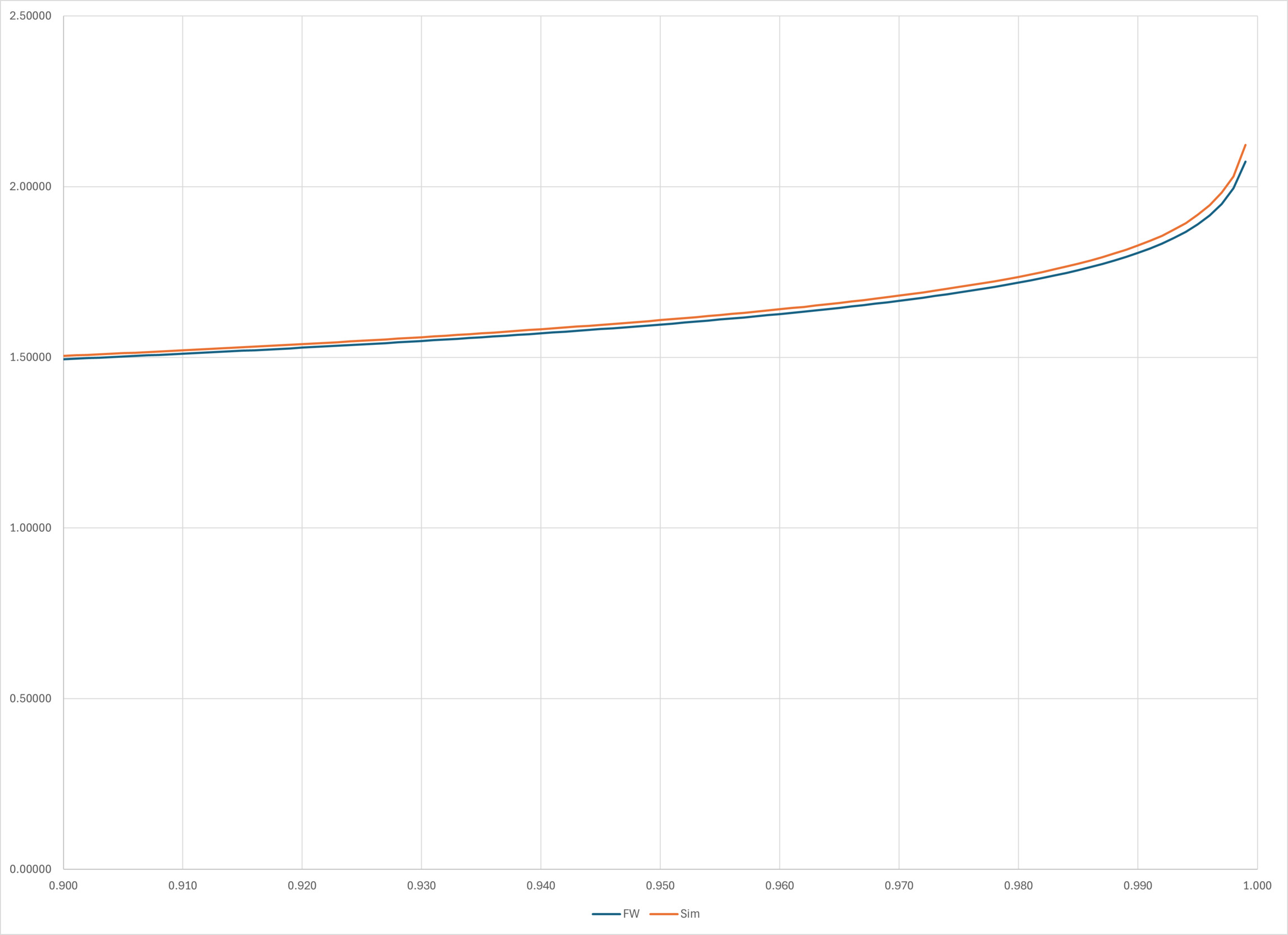
The simulated sum is simply the sum of these products. For this exercise, I simulated 1,000,000 sums, which give us an empirical distribution for the sum.[3] Denote the Fenton-Wilkinson approximation by and an empirical distribution based on simulated data by Equation 1 gives us the true mean dollar payment. The dollar amount of capital needed to support the payments at a 99.5% VaR level can be estimated by inverting each of the cumulative distribution functions of and and distributions and subtracting the expected payment, giving us two estimates:
ˆcFW=F−1FW(0.995)−856,289=1,170,663−856,289=314,374.
ˆcSI=F−1SI(0.995)−856,289=1,178,580−856,289=322,291.
These estimates would likely be considered close enough, for most purposes, so that either estimate by itself would be considered reasonable. Of the two, is unbiased, while is generally biased, though not by much, and is computationally simpler.
The example above did not admit any variation in the amount or timing of loss payments, which is of course unrealistic. For example, suppose we vary the scenario from the previous paragraph so that instead of paying €200,000 each year for four years, we must pay €800,000 at one of those times and zero at the others, with a 25% chance of payment at each time. The expected total value of payments in this scenario is the same as in the previous scenario, but the higher moments and quantiles of the distribution are not the same. Generally, unless our interest is very narrow, for example, if we are interested in only the mean of a stream of transactions and do not care about tail risk, we will have to model timing variations by producing separate distributions, with different sets of payment time weights, then creating a mixture distribution over the results. The basic point is that a weighted sum distribution is generally not the same distribution as a mixture distribution over the same random variables using the same weights.[4] Scenarios wherein payment occurs at only one of several possible times are relatively straightforward because the distribution of the exchange rate at each single point of time is lognormal and easy to find. For example, consider the scenario already described, with a payment being required at the end of one of years 1 through 4, with equal probability. The distribution of the exchange rate at each of these times is lognormal, with canonical parameters calculable with Equation 8 and the data in Table 4 and shown in Table 1, where represents the payment in EUR if one occurs at that time, and the categorical probabilities decide at which time payment occurs. What is the appropriate capital needed to support the market risk on this obligation at a 99.5% VaR level? If represents the current dollar equivalent of a payment when it occurs and represents the time of payment, then the cumulative distribution function of can be written as
FZ(z)=4∑t=1Pr(Z≤zθt∣τ=t)Pr(τ=t),
where is the USD present value factor from time This also can be written as where is the EUR payment at time discounted at the USD rate for that term. For example, To compute the inverse cumulative density function for a quantile we must locate a value such that which is easy by numerical methods. In this case, we find that [5] Subtracting the expected payment gives required risk capital of $543,711.
The method is relatively simple because payment will be made at only one time. Things are more complicated if we consider different scenarios, each involving payments that occur at different times. For each such scenario, we would have to use either simulation or the Fenton-Wilkinson approximation to estimate the distribution of possible payments. Then we would create a mixture distribution over the scenarios. While this is not technically much more difficult than the example already described in this paragraph, the computational resources required could be substantial if the distribution of payments for each scenario were estimated by simulation.
If the total amount due in foreign currency and the exchange rate are statistically independent, then any probabilistic variation in the total amount of payments simply scales the payment amount.[6] Thus, if is a EUR payment due at then is the random variable representing the dollar payment amount, whether is a fixed amount or a random variable. For a simple application, modify the scenario from the previous paragraph by supposing that the required payment is with probability and zero otherwise. This is the cumulative distribution function
F_{Z}\left(z\right)=\left(1-\frac{1}{3}\right)+\frac{1}{3}\sum_{t=1}^{4}m_{t}F_{X_{t}}\left(\frac{z}{2w_{t}}\right),
which yields The model of a lognormally distributed payment is particularly useful because it is a common model for loss payments and also because the product of two lognormal variables is itself lognormal. Thus, if it is believed that a payment in that will be required at time is lognormally distributed, and if the distribution of is lognormal as described by Equation 8, then the payment in follows the lognormal distribution
\small{ Z_{\tau}\sim\operatorname{Lognormal}\left(\ln\left(X_{i,j,0}\right)+\ln\left(\frac{1+r_{i,0,\tau}}{1+r_{j,0,\tau}}\right)-\frac{\sigma_{i,j}^{2}}{2}\tau+m,\sqrt{\sigma_{i,j}^{2}\tau+s^{2}}\right). \tag{2} }
Sometimes not all premiums, expenses, and loss are subject to foreign exchange market risk, but whichever ones are subject should be modeled together, on a net payment basis, because any given movement in exchange rates will tend to affect their values in offsetting ways. If premiums are going to be due when expenses must be paid, for example, then the risk of receiving less domestic currency in exchange for premium revenue may be partly offset by reduction in the domestic currency value of expense payments.
Reinsurers often write treaties that have terms denominated in domestic currency but that are nonetheless exposed to foreign exchange risk by virtue of foreign-covered risks. Even a domestic insurer, writing policies only in its home state and with losses, premiums, and other policy terms denominated in domestic currency, may face material foreign exchange risk, if, for example, loss settlement depends on imported parts or worldwide coverage is provided. The key considerations here are the sensitivity of payments to exchange rates and any censoring of payment amounts by policy deductibles and limits. A simple model for the domestic currency amount of loss is
Z_{\tau}=W_{i,\tau}+X_{i,j,\tau}W_{j,\tau}\tag{3}
\eta_{j}=\frac{E\left(X_{i,j,\tau}\right)W_{j,\tau}}{W_{i,\tau}+E\left(X_{i,j,\tau}\right)W_{j,\tau}},
where is the expected fraction of payments effectively denominated in the foreign currency (and the elasticity of the expected total payment in domestic currency with respect to the exchange rate) and is the expected amount of payment in currency A policy attachment point or deductible expressed in domestic currency units has the effect of truncating the left tail of the distribution of A limit that is expressed in domestic currency units has the effect of censoring the right tail of the distribution of For example, consider an insurance program written by a US insurer on Eurozone exposures, divided into aggregate excess of loss layers for reinsurance, with attachment and limit points specified in USD, on a risks-attaching basis, with a per-layer aggregate loss limit of $10,000,000, which attaches at $ to underlying aggregate loss on the exposures. Suppose aggregate loss from the exposures is lognormally distributed. Finally, suppose loss payments are remitted by the reinsurer in USD, but loss amounts ceded to the treaty are converted from EUR to USD using exchange rates as of the dates of occurrence.
Though payment is made in USD, the losses are mostly denominated in EUR; thus we can reasonably assume If the treaty incepts now, for one year, then the average date of occurrence for losses will be about one year in the future. If we accept this as an approximate date of occurrence for all losses and assume loss reports are made instantaneously, we can effectively simplify Equation 3 to and because we are assuming is lognormally distributed, this can be written, using Equation 2 and data from Sections 2 and 3, as
\scriptsize{ Z_{\tau}\sim\operatorname{Lognormal}\left(\ln\left(1.121\frac{1.0337}{1.0179}\right)-\frac{0.0262^{2}}{2}12+m,\sqrt{0.0262^{2}12+s^{2}}\right). \tag{4} }
For example, assume and so Equation 4 reduces to For a reinsurer with EUR as its domestic currency, the unlimited distribution of loss would be in EUR terms. Such a reinsurer would not worry about the actual exchange rate, because its assets’ values would move in concert with its treaty liabilities, but we need to convert its expected costs to USD to allow for comparisons to the USD domestic. For this, we can convert at the (fixed) expected exchange rate, which yields or The distributions from the perspectives of the USD domestic and EUR domestic have the same expectation, approximately $51.4 million, but different variance. The variance for the USD domestic is about 3.74% higher. The breakdown of expected aggregate loss by layer in USD terms is shown in Table 3.
Table 3 presumes that the entire program is divided into $10,000,000 aggregate layers and shows the expected loss from each layer to a reinsurer with USD as its domestic currency and to one with EUR as its domestic currency. Both sets of figures are shown in USD, but for “EUR Domestic,” the loss figures are converted to USD using the expected exchange rate as a nominal conversion factor. The risk of adverse exchange rate movements effectively stretches the right tail further to the right, raising the probability that upper layers will be pierced. For the USD domestic, this risk becomes substantial. Conversely, in low layers where there is a relatively high chance that some loss is payable, the USD domestic actually has a small advantage because with loss likely to be at the limit, there are fewer scenarios wherein adverse exchange rate movements can make things worse, while favorable exchange rate movements are relatively likely to make a beneficial impact.[7]
1.1. Regulatory and rating considerations
The treatment of exchange rate risk by the National Association of Insurance Commissioners (NAIC) is generally quite limited. The NAIC Annual Statement does not have exhibits that separately list insurance-specific reserves that are affected by foreign currency values or that represent obligations to foreign claimants. The Annual Statement does include a summary line titled “Net adjustment in assets and liabilities due to foreign exchange rates” in three places: row 22 of the Assets page, row 17 of the Liabilities page, and row 22 of the Exhibit of Nonadmitted Assets, but these have quite a narrow use. They are used to record only Canadian assets and liabilities, and only if they are small. The entries record unrealized gains or losses in the dollar value of assets net of liabilities that are denominated in Canadian dollars (CAD).[8] For example, suppose $1.37 million in CAD was purchased on July 1, 2024, when the CAD/USD exchange rate was 1.37, and then held in cash. At the end of the last trading day of the reporting period, December 31, 2024, the exchange rate was 1.44, and the USD value of this holding would have fallen to of its original value, or The (unrealized) drop in value, would have been recorded as a decrement to the value shown on row 22 of the Assets page if the total of such changes were greater than zero and otherwise on row 17 of the Liabilities page. This is a very limited purpose, and the entries on these rows are on average less than 0.1% of total assets and liabilities of property and casualty insurers.
Note 12 includes a more detailed treatment of some foreign currency assets and liabilities, but only those held as part of any defined benefit plans run by the insurer for its staff.
Owned foreign bonds are identified in Schedule D, and options, derivatives, and similar instruments that are affected by foreign exchange rates are identified in Schedule DB. These are generally the most significant entries relating to foreign currency in the Annual Statement, but they are given no special treatment other than specifying that bonds that pay a fixed coupon in a foreign currency should be treated as variable coupon bonds.
AM Best takes these entries, supported by a little more information from the Supplemental Rating Questionnaire, and generally applies an additional risk factor of 20% to foreign-denominated assets in the calculation of BCAR for US property and casualty insurers (over and above any other risk charge due to the asset category). Owning foreign-denominated assets would often not be a sensible means of hedging the risk of foreign property and casualty liabilities anyway, but this additional risk charge effectively ensures that it is almost never the case.
European insurance regulation is largely built around the Solvency II directive, which came into force in 2016 and considers exchange rate risk somewhat more carefully. In accordance with Solvency II, a European Union agency called the European Insurance and Occupational Pensions Authority (EIOPA) is tasked with providing various data used to value assets and liabilities, some of which are discussed below in Section 3. Solvency II takes a two-pronged approach to financial stability modeling, with some prescribed calculations, as in accordance with NAIC, and with a considerable emphasis on enhancing companies’ own ERM systems. The prescribed calculations produce two standardized capital requirements: the minimum capital requirement and the solvency capital requirement. These are intended to meet VaR 85% and 99.5% enterprise risk standards, respectively. The market risk module in the calculations includes a currency risk submodule that applies a fixed 25% risk charge to foreign-exchange-forward contracts. Individual companies are encouraged to be more sophisticated in their own modeling of exchange rate risk as part of their approach to ERM, and it would behoove any company subject to Solvency II and with potentially material foreign exchange risk to demonstrate that it has its own internal modeling of such risk.
1.2. Policy and reinsurance considerations
The impact of exchange rate risk on profitability may be either mitigated or enhanced by various policy and reinsurance features, including the following.
Setting policy limits in USD mitigates risk by insulating the maximum claim size from exchange rate risk. Even if limits are expressed in USD, however, claims below limits still may be affected by exchange rate changes if they are payable on a basis that varies with the value of foreign currency. For example, consider a property line where settlement is made at the lesser of repair cost or the policy limit. The USD cost of repairs will be proportional to the exchange rate into the foreign currency, so for losses that don’t hit the policy limit, the policy is affected by exchange rates as if the limit were expressed in the currency of the country where repairs are effected. Thus, one must consider the expected fraction of loss uncensored by the policy limit when evaluating exchange rate risk.
Note that in some lines, it is acceptable to market participants to express limits in a foreign currency but to state a fixed exchange rate in the policy. This is common in the Aerospace line, for example. The result is generally equivalent to setting a USD limit. In exceptional cases, there might be some slight risk of the foreign currency being unobtainable when payment must be made, but this is highly improbable and can matter only if payment must be made in the specified foreign currency.
Even if policy limits are expressed in foreign currency and the exchange rate is not fixed, the effect of having a USD limit may be afforded by excess of loss reinsurance that is fully placed and attaches at USD limits. If the placement is only partial, then the retained portion still will be subject to exchange rate risk in the excess layer, and if there is a possibility of losses exceeding the reinsured layer or exceeding the number of reinstatements, then exchange rate movements still may affect the amount of loss in the retained portions. Tredwell’s Fine Arts program is an example of a program that mitigates exchange rate risk very effectively in this way. Exposures written by this program are covered in whatever country they are located, and repair costs often depend on fees charged by the original artist, who may be located in any foreign country even if the insured items are in the US, so loss costs can clearly be affected by exchange rates. However, all loss greater than a fairly low per-occurrence attachment point is reinsured, and losses that do occur are likely to reach that attachment, so the retained part of loss is not materially affected by exchange rate changes.
2. Exchange rate volatility[9]
Across the span of modern history, there have been three common types of exchange rate regimes, which describe the degree to which exchange rate fluctuations are “controlled” by national or international public institutions. Fixed exchange rates are those that currency traders do not expect to change in the foreseeable future. They can be supported either by commodity-backed currencies (e.g., a “gold standard”) or by credible promises to use public policy to maintain the exchange rate if needed against market pressure. Pegged or semifixed exchange rates are backed by looser promises, which typically permit some small band of fluctuation. Floating exchange rates, as the name suggests, are determined at any time mainly by supply and demand for each of the currencies. Through most of its history up to 1971, most of US trade has been with countries whose currencies were effectively convertible at fixed rates to gold bullion and whose exchange rates were thus for the most part fixed. Some countries have since attempted to fix or peg their currencies against USD. For example, between 1991 and 2002, Argentina attempted to fix the Argentine peso exchange rate against USD. Such efforts have generally met with short-term success at best and are not really relevant for current projections. Most currencies now float against USD and are likely to do so for the foreseeable future.
The standard theory of exchange rate fluctuations between currencies that “float” against each other is based on a relationship called “interest rate parity,” which suggests that (absent various market imperfections) the difference between the current (spot) exchange rate and the forward exchange rate between two currencies (the rate that financial markets expect to pertain at some future date) should prevent arbitrage by compensating for the difference between local interest rates in each currency.[10] Risk of future fluctuations will remain, but in effect, risk-neutral market participants always should be indifferent between holding currency or The key relationship can be expressed for our purposes as
E\left[X_{i,j,t+\tau}\right]=\frac{1+r_{i,t,t+\tau}}{1+r_{j,t,t+\tau}}X_{i,j,t},\tag{5}
where is the spot exchange rate at time expressed as the number of units of currency that can be bought at time for one unit of currency and is a zero-coupon interest rate that can be earned in currency from time to
The random process underlying Equation 5 is readily and commonly modeled as a continuous geometric Brownian motion with constant volatility parameter that is, a stochastic differential equation of the form
dX_{i,j,t}=\left(\rho_{i}-\rho_{j}\right)X_{i,j,t}dt+\sigma_{i,j}X_{i,j,t}dW_{t},
where denotes the continuous, constantly compounding rate of interest equivalent to over the interval between and and is a Wiener process. This can be shown to imply
X_{i,j,t+\tau}=X_{i,j,t}\psi_{i,j,t,t+\tau}\;,
\psi_{i,j,t,t+\tau}\sim\operatorname{Lognormal}\left(\left(\rho_{i,t,t+\tau}-\rho_{j,t,t+\tau}\right)\tau-\frac{\sigma_{i,j}^{2}}{2}\tau,\sigma_{i,j}\sqrt{\tau}\right).
Using the relationship we can express the random variable as
\psi_{i,j,t,t+\tau}\sim\operatorname{Lognormal}\left(\ln\left(\frac{1+r_{i,t,t+\tau}}{1+r_{j,t,t+\tau}}\right)-\frac{\sigma_{i,j}^{2}}{2}\tau,\sigma_{i,j}\sqrt{\tau}\right).\tag{6}
Note that so Equation 5 is satisfied. Taking logs and rearranging gives
\ln\left(X_{i,j,t+\tau}\right)-\ln\left(X_{i,j,t}\right)-\ln\left(\frac{1+r_{i,t,t+\tau}}{1+r_{j,t,t+\tau}}\right)+\frac{\sigma_{i,j}^{2}}{2}\tau=\varepsilon_{i,j,t,t+\tau},\tag{7}
where As is a constant, we also have
\small{ X_{i,j,t+\tau}\sim\operatorname{Lognormal}\left(\ln\left(X_{i,j,t}\right)+\ln\left(\frac{1+r_{i,t,t+\tau}}{1+r_{j,t,t+\tau}}\right)-\frac{\sigma_{i,j}^{2}}{2}\tau,\sigma_{i,j}\sqrt{\tau}\right).\tag{8} }
We can use actual spot exchange rates and interest rates over time to estimate the volatility term Various interest rates and terms could be used, but it is usual to select rates that are as close to risk-free rates as available in each currency, with short terms and many recent nonoverlapping observation periods for both currencies. Overnight interbank lending rate data are suitable and readily available for most major currencies, reported at least monthly. Exchange rate data are usually available on daily and monthly bases and sometimes more frequently. In practice, though it is usual to assume that is constant, we must acknowledge that there are occasional episodes of greater volatility from which we should sample, if possible, to avoid making biased projections. This is particularly important given that for the purposes of modeling insurance risk, we are usually interested in projections over as many as 10 years or more. As a target, monthly data from a historical period of 10 to 20 years will typically suffice. With careful consideration, however, other datasets will be perfectly usable. Assume we assemble a dataset from normalized times to in unit increments and use the notation
\epsilon_{i,j,t}=\ln\left(X_{i,j,t+1}\right)-\ln\left(X_{i,j,t}\right)-\ln\left(\frac{1+r_{i,t,t+1}}{1+r_{j,t,t+1}}\right).
The usual estimate of from this data is the sample standard deviation of the :
\hat{\sigma}_{i,j}=\sqrt{\frac{1}{T-1}\sum_{t=0}^{T-1}\epsilon_{i,j,t}^{2}}.
Note that is a constant, so excluding it from the definition of does not bias its second central moment.
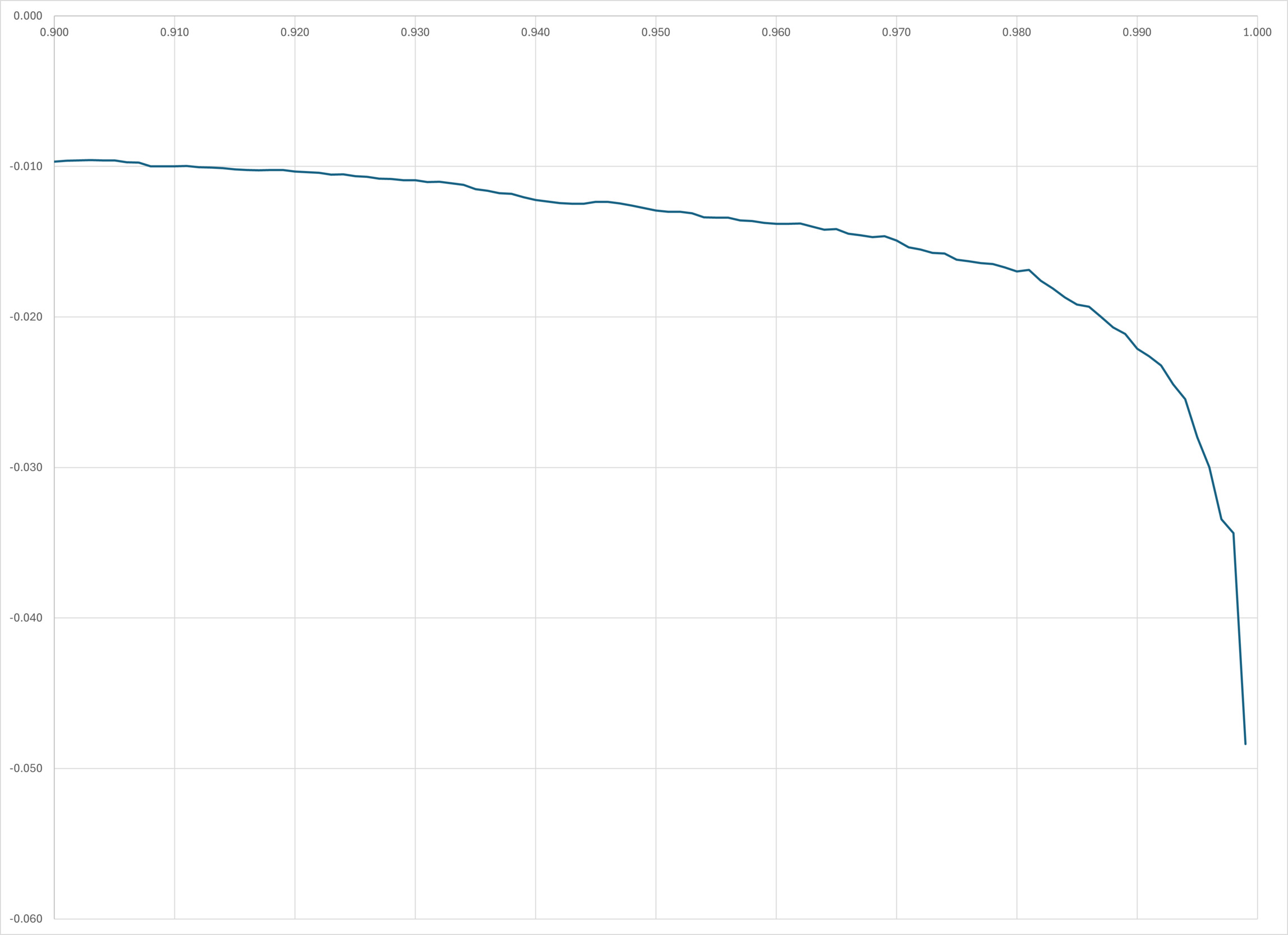
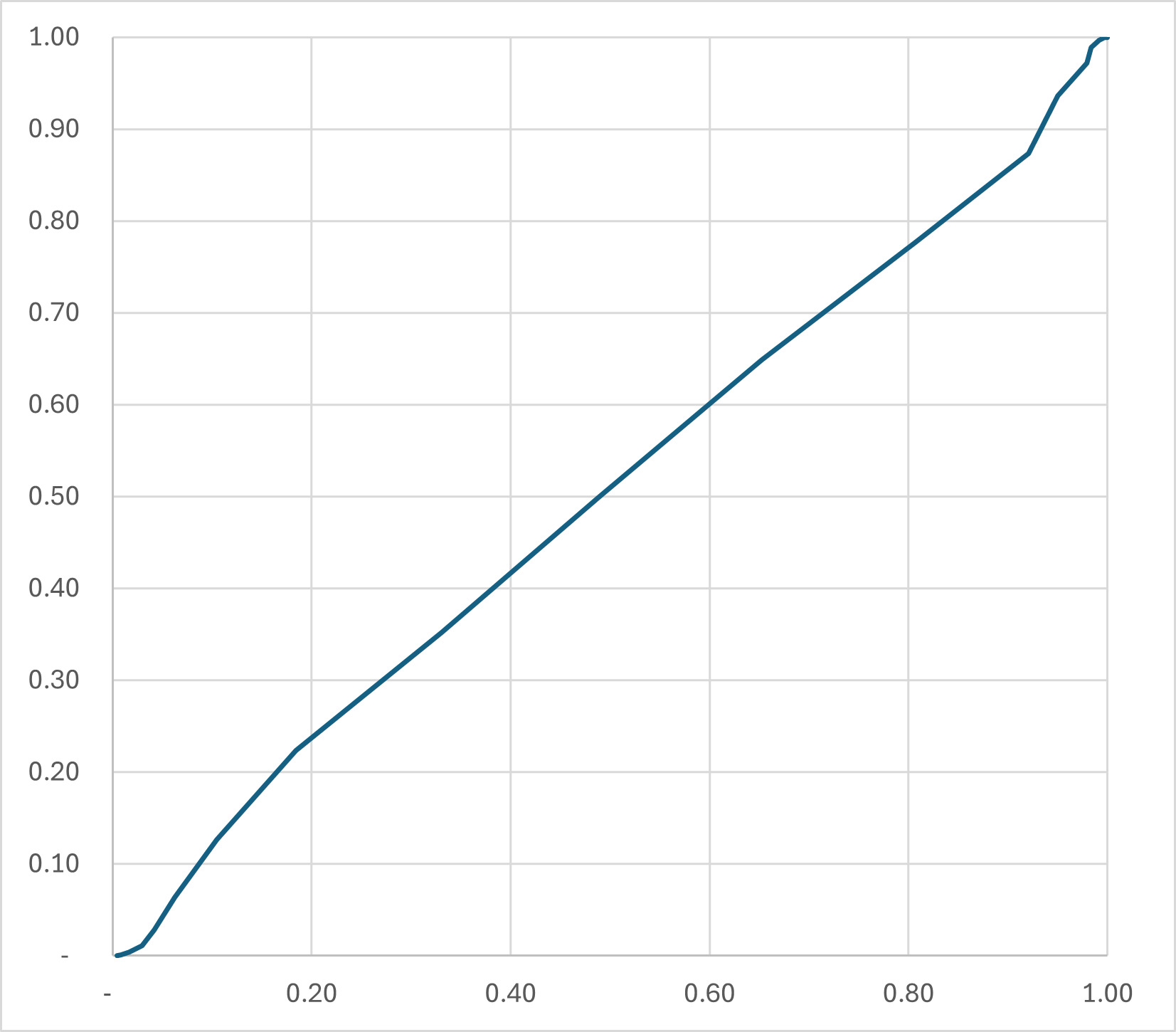
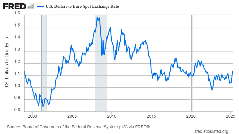
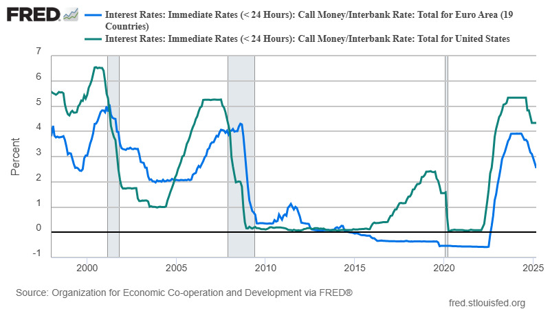
For example, consider the daily close of the USD/EUR exchange rate, shown in Figure 2.[11] The relevant USD and EUR interest rates are shown in Figure 3.[12] The EUR is a fairly new currency, and the period before 2005 is best ignored as financial markets took until around then to decide what to make of it. The period between 2008 and around 2012 was affected by the Great Recession, which may have affected volatility in unusual ways. Table 4 shows the beginning and ending rows of a table of data from 20 years, a total of 239 rows. The columns US/EU show spot exchange rates at the “begin” and “end” dates, respectively. “Rate US” and “rate EU” show the overnight lending rate for each currency area at the “begin” date. “Error” shows the error term calculated according to Equation 7.[13] The sample standard deviation of the epsilon terms is Next, we should check that the errors are sequentially independent. Fitting an AR(1) model to the data gives an estimated coefficient of with a parameter standard error of so clearly there is no significant autocorrelation. We should also check the mean of the epsilon terms. In this case the mean is which is not significantly different from Finally, we can inspect the distribution of errors to check for nonnormality. Figure 4 is a “PP” plot, showing the cumulative distribution function of the actual errors on the horizontal axis against the cumulative distribution function of the fitted normal distribution on the vertical axis.
The fitted line is more or less straight from lower left to upper right, with short flatter sections at each corner. These flatter sections indicate that the distribution of projection errors has somewhat fatter tails than the fitted normal distribution, perhaps because we included data from the period of crisis around the Great Recession. If nonnormality is a serious concern, then we can use a stochastic model based on something other than a Wiener process, such as a distribution with jumps or even the empirical distribution from our dataset; however, alternatives such as these commonly require more data to achieve a good fit, without which they can mislead in other ways. I think the normal assumption will typically be reasonable.
2.1. Other theories of exchange rate movements
The theory of interest rate parity supposes that investment returns are generally equal in different countries with floating exchange rates. Another important theory of exchange rate determination is purchasing power parity (PPP), which posits a close relationship between prices of goods and services in different countries. The theory is that similar products should have similar prices in different places, so exchange rates should subsist at levels that make prices roughly equal, regardless of location. The posited relationship is “close” rather than exact because the theory admits that local prices can be affected by differing transport and storage costs, tax differences, lack of availability of exactly similar products, and various other geographic variations. It is generally hard to test whether purchasing power parity pertains, not only because the variations already mentioned are hard to quantify but also because price indexes are generally not exactly harmonized between countries. Nonetheless, suppose data are found that suggest parity does not hold. Say, though EUR/USD is 1.121, it is found that a basket of goods that costs $100 in the US costs €91.70 in the EUR area. PPP suggests that EUR/USD should be It could be inferred that EUR is overvalued in terms of USD by 2.8%. Such information can be useful and does sometimes suggest future exchange rate “corrections” that for some reason are “missed” by interest rate parity, but projections based on PPP should be scrutinized with great care. At best, studies using PPP are generally limited to current exchange rate imbalances and say little about how quickly we can expect any corrections to occur—some price imbalances seem to persist for a very long time.[14]

The field of behavioral finance has given rise to some other theories of exchange rate movement. Behavioral finance seeks to augment traditional finance models by modeling various cognitive and emotional biases, such as herd behavior, overconfidence, and conservatism, to account for apparent market anomalies. Behavioral finance is not a single integrated theory but a collection of separate models that can be applied piecemeal, and it takes considerable knowledge and judgment to do so effectively. In backward-looking models that seek to explain historical episodes, this work often produces persuasive results, but good forward-looking projections are more rare.
Overall, I would say that while alternate theories of exchange rate movement may be considered, and may on occasion indicate a particular need for caution, most exchange rate projections should rest primarily on results from interest rate parity models.
3. Exchange rate projections
To model future exchange rate risk, we need the modeled volatility term from above, and also an estimate of the expected trajectory of the exchange rate, also known as a foreign exchange or FX forward curve. There are several ways to obtain such estimates.
One of the easiest, where available, is to observe expected future exchange rates directly, from reported or quoted foreign exchange forward transaction data. However, market transaction and quote data are not readily available for all currency combinations, especially “minor” currencies. Moreover, pricing typically reflects asymmetric need for the trade—the “buyer” typically gets a “worse” deal than the “seller.” This is exemplified by “bid-ask” spreads in quote data. Finally, some currency markets are thinly traded, especially at long forward maturities, and prices can be materially affected by even slightly unusual demand.
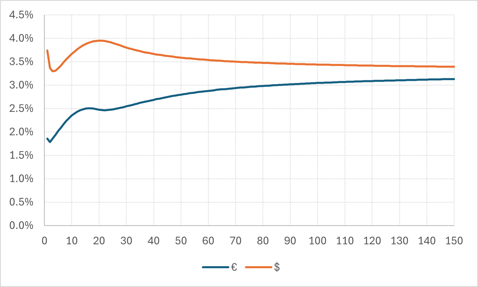
Another way to obtain an FX forward curve is to use the current exchange rate and yield curve data for each currency to project the ratio of interest factors in Equation 5. This is how trading firms that do a lot of forward currency trades typically set their own prices. Yield curves require interest rate data for various maturities, and such rates in some currencies can be hard to obtain. Estimating “zero-coupon” yields to fixed maturities also may be difficult. Where available, it makes sense to use yield curves prepared by third parties. A good source for calculations relating to insurance liabilities is EIOPA, which publishes term structure data for this precise purpose, as described in the Solvency II directive.[15] The EIOPA data reflect some conservative modeling choices, as might be expected from an insurance regulatory agency, but they are reasonable. EIOPA publishes various series monthly. The basic risk-free rate curves with volatility adjustment are generally suitable. EIOPA publishes spot rates from 1- to 150-year maturities for the currencies shown in Figure 5.

Because consistent modeling choices are carefully made when producing the yield curve for each currency on this list (see Dufresne 2009 for details), it should be used as a source for both currencies wherever possible. For example, consider risk-free spot rates listed in the April 2025 data release by EIOPA for the EUR area and the US, as shown in Figure 5. Interpolation and extrapolation are carefully applied to extend these curves in annual increments to any maturity that might reasonably be required by an insurer, even with long-term life or pension business.
EIOPA data are not available for many developing economies, and not even for all Organization for Economic Cooperation and Development countries. For other countries, other data sources must be found. Reliable term structure data are available from several sources, for example, the Federal Reserve Bank of St. Louis, but are typically available for only a few maturities, and a method of interpolation or extrapolation will generally be needed. There are many reasonable methods of interpolation and extrapolation. The most commonly used is probably the Smith-Wilson method described in Dufresne (2009), but the complexity of that method is often excessive unless it is required by external authorities. For internal risk management purposes, linear interpolation between known spot rates and extrapolation to an assumed fixed ultimate spot rate will generally be as good (Smith-Wilson differs from this only in assuming a form of smoothed spot-rate curve).
For example, at the time of writing this, which we will call month the EUR/USD exchange rate is 1.121, and the 12-year maturity rates listed by EIOPA are 2.431% for EUR and 3.767% for USD. Substituting into Equation 5 gives us
E\left[X_{i,j,t,t+144}\right]=\left(\frac{1+0.03767}{1+0.02431}\right)^{12}1.121=1.3096.\tag{9}
We can then substitute into Equation 6 to give
\scriptsize{ \psi_{i,j,t,t+144}\sim\operatorname{Lognormal}\left(12\ln\left(\frac{1+0.02431}{1+0.03767}\right)-\frac{0.0262^{2}}{2}144,0.0262\sqrt{144}\right),\tag{10} }
from which we can produce confidence intervals about For example, the confidence interval for reflecting a 1/250 event in each tail (between cumulative quantiles 0.004 and 0.996) is Table 3 shows further upper percentile values of the projected exchange rate distribution at different terms in years. This reflects quite extreme risk, corresponding to the 99.6 VaR calculations typically used by AM Best, and a very long term from a property and casualty perspective. Other confidence intervals, and intervals for other maturities and countries, can be derived in the same way. For an internal ERM analysis, I would recommend using this method with a confidence interval corresponding to whatever level of adverse shock is presumed elsewhere in the analysis.
In practice, the risk to be evaluated may stem from a series of expected payments or receipts over time rather than at one particular time, and this poses a practical computational problem. For a simple example, suppose a book of business is expected to produce €2 million of expected, payable in EUR, half of which is expected to be payable 12 months from now, with the other half payable 12 months later. Assuming currency is converted from USD for these payments at the time they become payable, what is the distribution of the USD value of total payments? The expected total payment is simply the sum of the expected payments at each time, that is, of €1 million after one year and €1 million after two years. We could use the approach shown in Equation 7 to find the distribution of the dollar amount of either one of the payments, which will be lognormal. The distribution of the sum of the payments is thus a variable whose distribution is that of a sum of two lognormal variables. The sum of lognormal variables generally does not exactly follow a lognormal distribution, and in fact remarkably little is known about the exact distribution of sums of lognormal variables. Certain approximations can be useful, and numerical methods also can be used. See Appendix A for further details.
4. Conclusions
It’s generally impractical for property and casualty insurers to hedge currency risk. The liabilities (and sometimes assets) whose risk would need to be hedged are typically of uncertain amount and duration, and our knowledge of these quantities does not generally develop smoothly, so a perfect hedge would be impossible. The amounts involved, in both dollar terms and duration, are often large enough to present serious practical difficulties, and the transaction costs involved in what could be quite long-term hedging strategies would be substantial. Moreover, any instruments held as part of a hedging strategy would typically incur large risk capital charges in the AM Best BCAR formula, which for most companies with international exposure is likely to be a very serious concern. The alternative is to manage the risk by modeling, measuring, limiting, and pricing it, and this paper shows how, without too much difficulty, property and casualty insurers can do so.
Most exchange rate models assume that exchange rates follow a geometric Brownian motion process with varying drift over time, with the result being that the distribution of an exchange rate at a future point in time, say when a loss may need to be paid, is lognormal. The expected present value of a sum of loss payments in a foreign currency at various future times can thus be represented as a sum of lognormal variates, which are of course correlated because they are derived from a single Brownian motion process. The sum of lognormal variates generally has no known analytic representation but is commonly modeled using either simulation or the Fenton-Wilkinson approximation, which fits a lognormal distribution to the sum, usually by a method of moments. Appendix A develops a method-of-moments Fenton-Wilkinson approximation for a sum of lognormal distributions that are all point-in-time distributions from a geometric Brownian motion process such as an exchange rate, and it compares this approximation under reasonable conditions to results achieved by simulation. The Fenton-Wilkinson approach is slightly biased but computationally simpler, and the amount of bias is unlikely to be of practical concern in the context of an insurer managing exchange rate risk, so I would generally recommend this approach.
The varying drift of an exchange rate process is typically modeled by applying the assumption of covered-interest parity, which is that risk-free interest rates payable in each currency should produce the same rates of return after exchange into any common currency, in expectation. The expected path of exchange rates thus can be modeled using yield curve data for each currency. Section 3 explains how yield curve data from EIOPA can be used for this. EIOPA data are not available for all currencies, and some alternate data sources also are discussed. Modeling the volatility of an exchange rate process generally can be done by using historical data on actual exchange rate movements, as explained in Section 2. Section 2 also includes a brief discussion of the theory of PPP, which in certain circumstances may usefully augment the projections found using covered-interest parity.
Section 1 gives simple examples that show how exchange rate risk can affect the value of an asset or an insurance liability and how this can be managed using the tools described in this paper to measure risk exposure using standard metrics such as VaR. Exchange rate risk is not always obvious. Under certain circumstances, it even can affect an insurer that writes policies only for insureds located in its domicile and for premiums denominated in its domestic currency, for example, if repair costs require imported parts or if insureds are covered wherever in the world they may be. Section 1 also explains some important limitations on the treatment of exchange rate risk by regulatory models and rating agencies.
_distributions.png)