When a Portfolio Reaches Sufficient Scale

1. Introduction

It is common, particularly in severity-driven lines of business, to believe that a new book of business needs to reach “scale”—that is, sufficient size to absorb an unfortunate loss or two. While this concept makes intuitive sense, as it is clearly easy for a single large loss to wipe out the premium of a small portfolio, there has not yet been a mathematical framework to support the concept of “scaling.” This paper articulates one such framework and its implications.

1.1. Research context

The concept of book scaling is predominantly a risk management idea. Anyone who has shepherded new books of insurance in the early stages knows the risk, if not the experience, of early large loss activity. I am not familiar with any material that addresses this business consideration from an actuarial framework. However, in preparing this analysis, I have reviewed and relied on common portfolio modeling assumptions. In particular, I based my frequency and severity framework on “Modeling Insurance Frequency with the Zipf-Mandelbrot Distribution” (Dalton et al. 2022).

1.2. Objective

There is currently no mathematical framework for the common insurance concept of scaling, and neither are there metrics by which to measure it. This paper will propose such a framework and a measurement approach.

1.3. Outline

The remainder of the paper proceeds as follows. Section 2 will discuss the assumptions made for theoretical books of business. Section 3 will illustrate the effects as a book grows and suggest a possible use case. Section 4 will briefly conclude by presenting the results.

2. Background and methods

When an insurance company writes a new book of business, it is, particularly in the early stages, exposed to plain and simple bad luck. This is even more true for a line with high severity and low frequency; assuming otherwise adequate pricing, a severity-driven book is less predictable over the short term. This phenomenon creates a discussion point around a book that has not yet reached, or needs to reach, “scale.” But what are the mathematical underpinnings for this argument? And how does one know when a book has indeed attained “scale”?

As makes intuitive sense, the dispersion around mean loss decreases as the book scales up. This reduced dispersion is desirable for a variety of reasons. Assets with lower volatility are explicitly more desirable in a capital asset pricing model. Similarly, both in the context of actuarial pricing and in general, more information is preferable to less information. Last, lower volatility preemptively curbs the possible effects of overreactive decision-making in the presence of a large loss.

A standardized measure of dispersion is the coefficient of variation (CV). This dimensionless property allows comparison of the variability of loss ratio, regardless of the portfolio’s size or propensity for loss. As a simple first example, assume a book with Poisson frequency and scalar severity. Besides the well-known properties that make the Poisson easy to work with, it’s often assumed for frequency distributions, including the useful and popular Tweedie model. In a severity-driven book, small (attritional) losses have negligible impact on profitability, so assuming all losses are limit losses is a reasonable simplification. We then calculate the CV using the following terms:

• Book premium = P (in $1,000,000s)

• Frequency (claims per $1,000,000 earned premium) = F

• Severity = S

Then we can calculate

$$\text { loss ratio mean }=F \times P \times S / P=F \times S \text{.} \tag{2.1}$$ (2.1)

In a compound Poisson distribution, the variance of loss is the Poisson’s mean multiplied by the second moment of the severity. Thus, the variance is

$$\text { loss ratio variance }=F \times P \times S^2 / P^2=F \times S^2 / P \text {.}\tag{2.2}$$

Because the premium is fixed, it can be pulled out of the remaining variance calculation as the inverse of its square. Finally, we can determine the CV:

$$\text { loss ratio } \mathrm{CV}=\left[F \times S^2 / P\right]^{0.5} /[F \times S]=[F \times P]^{-0.5} \tag{2.3}$$

This value is independent of the severity; it is strictly a function of the frequency and the book’s size, equivalent to the predicted claim count. After we define a few more terms, we can rearrange Formula 2.3 in a of couple ways. Let us define two more terms:

• Average policy premium = A (in $1,000,000s)

• Target CV = T

Thus, we can rearrange the formula in two ways

$$\text { target premium }=1 /\left[F \times T^2\right] \tag{2.4}$$

$$\text { target policy count }=1 /\left[A \times F \times T^2\right] \tag{2.5}$$

Using this simplistic framework, we can use Formulas 2.4 and 2.5 to calculate a target premium and policy counts given a target CV for a “frequency” book and a “severity” book:

Rows 2 and 3 of Table 1 are calibrated to realistic targets. A CV equal to 0.20, for example, is the same as exceeding an expected loss ratio of 60% by 12% at the 84th percentile (one standard deviation above mean). Similarly, row 3 is equivalent to exceeding an expected loss ratio of 60% by 4.6%. As 5% is a typical profit load assumption, this calculation calibrates the target around the probability that the book will not lose money. It should also be noted here that in each of these examples the expected loss ratio is 60%, which follows directly from the frequency and severity assumptions (per Formula 2.1). As expected, the challenge of taming variability is much more formidable with a low-frequency, high-severity book. Additionally, note that the scalar severity assumption in this framework is not particularly realistic for a typical “frequency” book, which can be expected to have a wide dispersion of claim severities contributing to its total loss.

These results can be generalized by using, for example, a zero-inflated Poisson distribution for frequency and/or a gamma distribution for severity. These distributions were selected for their common usage, but there is certainly no particular limitation to them. Recall the formula for the variance of an aggregate loss model:

$$\text { Variance }=E[F] \times \operatorname{Var}[S]+\operatorname{Var}[F] \times E[S]^2 \tag{2.6}$$

In Table 2, Formula 2.6 is applied to some possible combinations of frequency and severity assumptions. The third column is the CV for a given book size (by premium), while the fourth column contains the policies required to attain a CV of target = T. Two final definitions are required for terms in the zero-inflated Poisson and gamma distributions:

• Zero inflation to Poisson frequency = π

• Gamma distribution shape parameter (alpha) = α

Table 2 is included to demonstrate a range of book scales. As a reminder, these calculations benefit from a scalar premium value at a given book size, which is not a random variable and allows some simplification of the final result. While these formulas may seem cumbersome, recurring terms such as the base frequency assumption and adjustment for zero inflation or shape parameters drive recurring similarities. Note that for the zero-inflated Poisson frequency with a scalar severity, the CV matches a target T when

$$\text { policy count }=1 /[F \times A] /\left[T^2-T^2 \times \pi-\pi\right]. \tag{2.7}$$

The final term in this formula must be greater than 0; therefore, we can pull this term out and solve for the zero-inflation term given a target CV:

$$\pi<1 /\left[1+T^{-2}\right]\tag{2.8}$$

The frequency of limit losses already being thin, this calculation makes the zero-inflation term even harder to estimate. Therefore, I have left any potential enhancement by the inclusion of this term for future study.

3. Results and discussion

As the concept of book scale is usually focused on high-severity portfolios, the remainder of the paper will focus on the first and simplest framework using a range of assumptions. Returning to Table 2, we see that the target policy count depends on three characteristics:

• Average policy premium = A (assume $150,000)

• Frequency (claims per $1,000,000 earned premium) = F (assume 0.5)

• Target CV = T (assume 0.2)

These terms are listed roughly in order of availability, with the average policy size easiest to estimate and the target CV most subject to judgment. Table 3 articulates varying ranges around the baseline values assumed above.

The baseline assumptions are shown in bold in the first row. The target CV (column 3) uses the widest range around baseline, but even with this caveat, it’s clear that the results are very sensitive to this assumption. Thus, risk tolerance is a significant driver of a target book size. The baseline of 0.2 reflects a standard deviation of 12% on an expected loss ratio of 60%, a reasonable threshold for risk tolerance.

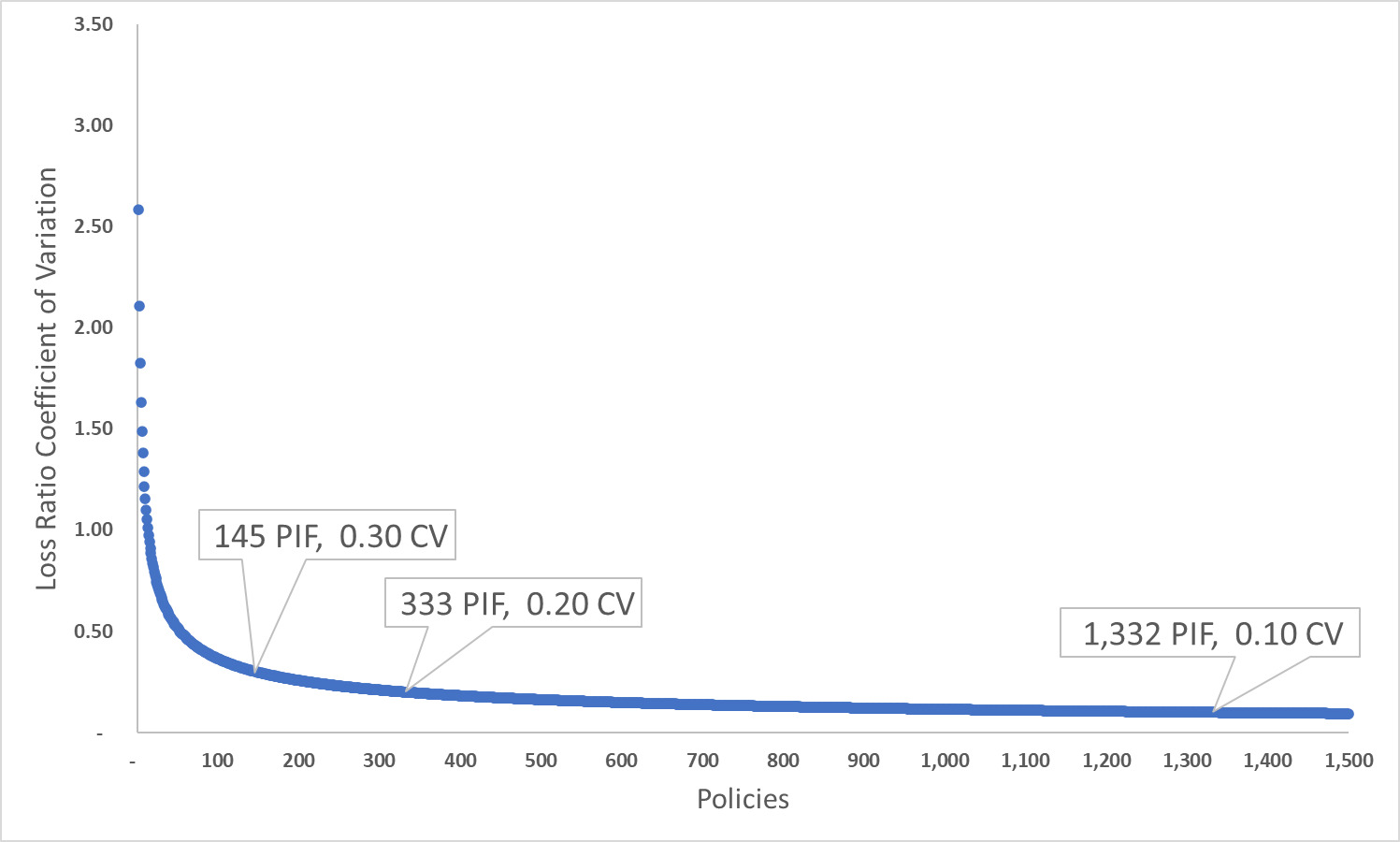
Since there is nothing magical about a specific CV, another way to consider a target value is depicted in Figure 1, which shows the target value’s relationship to policy count. The function is a power curve, dropping precipitously through the first 100 or so policies. On this basis, it could also be argued that 50 to 100 policies significantly ease the book’s growing pains, thereby helping it to attain scale.

Figure 1.CV by policy count (A = 150,000; F = 0.5).

PIF = policies in force.

To discuss the framework’s practical applications to limit tolerance, consider another book with these characteristics:

If we further assume an average limit of $5,000,000, from Formula 2.1, we get an expected loss ratio of 65%. As the book grows, there emerges a question of when it can assume higher limits without sacrificing average loss ratio or experiencing book volatility. Reinsurance is one possible solution, but given the possible barriers of added expense or market constraints, it will be left as a future consideration.

Fixing expected loss ratio and target CV, we can then calculate a wide range of scenarios using Formula 2.5. The starting point is highlighted in bold in Table 5.

By replacing frequency with an equivalent severity, Table 5 represents how to maintain a constant expected profitability and volatility under conditions of changing maximum loss or policy premium. Such a grid could be a guideline for keeping a book stable even as, for example, the average policy size increases to compensate for higher limits. This charge for increased limit could also easily be calibrated to market conditions.

4. Conclusions

Given the ubiquity of the belief that a new portfolio must attain a certain scale to absorb large claim activity, it is helpful to provide an actuarial perspective. The proposed framework can be adapted to a variety of assumptions and can support a practical threshold for scale. Thus, I believe this framework fills a gap in the actuarial and risk management tool kit.