Credibility as Data Augmentation

1. INTRODUCTION

1.1. Business Context

Insurance is all about volatility. The insurer takes on the risk of a financial loss from a policyholder in exchange for a set premium. The insurer can diversify this risk (somewhat) by “pooling” a portfolio of risks that are not 100% correlated; but the risk can never be fully diversified. Because of this inherent volatility, there will rarely be sufficient data to be fully confident in the estimation of the needed premium. Credibility theory helps by allowing the insurer to incorporate other data into the risk model.

Insurers often have “prior” estimates of the loss expectation. In ratemaking, this would be the current rating plan that is being updated with the latest data. In reinsurance, the prior information might be the expiring treaty, to be updated for new information in the renewal submission.

Even where the actuarial task is not explicitly updating an existing estimate, external data is often available. For example, an actuary working in Excess & Surplus lines may make use of the greater volume of loss data in the admitted market, albeit with a heavy dose of judgment to adjust that data for the different risks in the specialty market.

1.2. Definition of Data Augmentation

The present paper will highlight one way of including prior knowledge into an actuarial estimate, namely credibility as data augmentation. The concept of data augmentation is that we can combine our observed data with pseudo-data drawn from other sources. The pseudo-data is combined with the actual observed data, such that the actuarial model is applied to the augmented data set.

Data augmentation provides an alternative way of interpreting traditional credibility models and suggests new ways of implementing credibility in insurance applications such as ratemaking and size-of-loss curve fitting.

1.3. Historical Background

The idea of incorporating prior knowledge in the form of pseudo-data can be derived from Bayesian Statistics. Specifically, when using conjugate priors, data augmentation is equivalent to performing a full Bayesian analysis.

Bayesian Statistics has been the foundation of Credibility Theory beginning with Bailey (1950). Jewell (1974) showed that the linear “N/(N+K)” credibility formula was an exact Bayesian result when the statistical distributions came from the natural exponential family and related conjugate prior – but that the credibility form represented the best linear approximation even if the underlying distribution was not known.

The “N/(N+K)” form was extended in Bühlmann-Straub^[1] (1970) to allow for different exposure measures to be included. Bühlmann-Straub followed an “Empirical Bayes” format, wherein the complement of credibility was based on an overall mean, rather than from external information, but the mathematical form is the same.

A key challenge in applying this formula has been the estimation of the credibility constant “K .” The usual definition of K is the ratio of expected process variance (EPV or “within” variance) to the variance of hypothetical means (VHM or “between” variance). This definition is not so easy to grasp intuitively, nor is it easy to apply in practice.

An alternative method of calculation of the constant K was offered by Howard Mahler (1998), who proposed estimating the parameter based on minimizing the predictive error for a hold-out data set. Mahler’s approach is very similar to how a data scientist might estimate a smoothing parameter using cross-validation. In practice, this may work in only a limited number of cases where a data set is particularly robust.

For data augmentation, Huang et al. (2020) offers a few methods for estimating the weight to apply to the prior pseudo-data, including minimizing prediction error on out-of-sample data similar to the approach proposed by Mahler.

Recent work on incorporating prior data in a Bayesian model is the “power prior” approach introduced in Ibrahim and Chen (2000) and described more fully in Ibrahim et al. (2015). The original applications related to medical treatments (e.g., AIDS, cancer), where data from prior trials was available. The weight assigned to the data from prior studies could either be fixed by the analyst or treated as a random variable whose distribution is estimated by the model.^[2]

The method of data augmentation does not solve the estimation problem. However, it does give an interpretation of the credibility constant as the volume of pseudo-data added to augment the observed data. Credibility is a form of “borrowing strength” and the credibility constant, K, is an answer to the question “how much strength do you want to borrow?” How much additional data would you want to have?

Data augmentation is not limited to Bayesian models. It is closely connected also to classical models such as Ridge Regression (Hoerl and Kennard (1970) and Allen (1974)).

1.4. Objective

The goal of this paper is to provide a description of credibility as data augmentation. There are two advantages to this approach:

• It provides an intuitive physical meaning for the credibility constant.

• It provides an alternative method for incorporating prior information into an actuarial analysis.

Like the familiar N/(N+K) formula, the data augmentation result is exactly equal to the Bayesian results in the case of conjugate prior relationships but provides a useful blending of prior information even if loss distributions are not explicitly defined.

1.5. Outline

The remainder of the paper proceeds as follows.

Section 2 – General Examples of Data Augmentation

Sect 2.1 Thomas Bayes’ thought experiment

Sect 2.2 Ridge Regression

Sect 2.3 Generalized Linear Models (GLM)

Section 3 – Insurance Example on Size-of-Loss Curve-Fitting

Section 4 – Conclusions

Appendix – Practical Principles for Setting Credibility Standards

2. Selective examples of data augmentation

We proceed to give a very selective history of the use of data augmentation in various applications. These examples are meant to help illustrate the ideas. The first two examples illustrate the concept generally; then the GLM can be applied for insurance ratemaking. A fourth example using Curve-Fitting is very specific for insurance losses and will be addressed in Section 3.

2.1. Thomas Bayes’ Thought Experiment

The first example is taken from Thomas Bayes’ “An Essay towards solving a Problem in the Doctrine of Chances”, edited and published (1763) by his friend Richard Price. The goal of the essay was to quantify “inverse probabilities.” That is, how to estimate the probability of some state of the world having observed some experimental data.

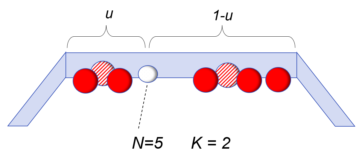
To address this problem, Bayes set up a thought experiment for randomly rolling balls on a long table. In the initial set-up, a white ball is rolled on the table in such a way that it could randomly land anywhere with equal probability; and its position is unknown to the experimenter. In the second step, a number of red balls are rolled on the table – also randomly and with their exact locations not told to the experimenter. The only information available is how many red balls, P, are to the left of the white ball, and how many, Q, are to the right of the white ball.

Figure 1.1.Bayes’ Thought Experiment

Knowing only the numbers P=2 and Q=3, can we make a statement about the probability that the white ball is between any two points X1 and X2? For example, what is the probability that u is between .40 and .50? Bayes gave an answer to this by estimating a series expansion for what we would now recognize as a Beta Distribution.

\[Prob\left( X1 \leq u \leq X2|P,Q \right) = \frac{\int_{X1}^{X2}{u^{P} \cdot (1 - u)^{Q}\ du}}{\int_{0}^{1}{u^{P} \cdot (1 - u)^{Q}\ du}} \tag{2.1.1}\]

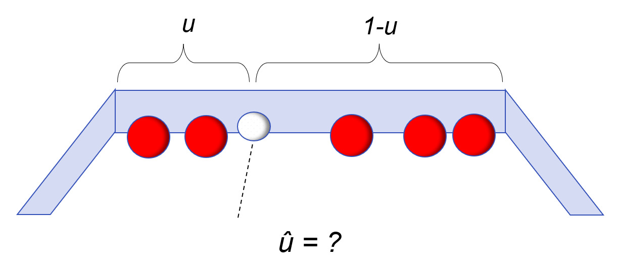
If we want a point estimate of the parameter u, representing the position of the white ball, we could use what we would today call the maximum likelihood estimator (MLE), being the ratio of the balls on the left, P, to the total number of balls N=P+Q. The MLE works well when P and Q are large numbers but can be misleading in small samples when, for example, P or Q are equal to zero.

\[{\widehat{u}}_{MLE} = \frac{P}{P + Q} \tag{2.1.2}\]

The alternative proposed by Bayes and Price would be the expected value of the Beta Distribution given as below.

\[E\left( u|P,Q \right) = \frac{P + 1}{P + Q + 2} \tag{2.1.3}\]

In our example, we would estimate u=3/7 based on this formula, not as 2/5 from MLE.

If a very large number of balls are rolled, such that both P and Q are large numbers, then these two estimators are very similar. But in “cases where either P or Q are of no considerable magnitude” (Price’s words) there can be big differences.

Unlike the maximum likelihood estimate, the conditional expected value never reaches either 0 or 1. Even if all of the red balls are to the right of the white ball, we do not estimate u=0.

The additional 1 in the numerator and the 2 in the denominator act as additional ballast and are based on the “prior knowledge” that the white ball was equally likely to have landed anywhere on the table. Spiegelhalter (2021) notes the connection to data augmentation because the prior knowledge can be viewed as “imaginary balls”, one on either side of the line separating left and right.

“In fact, since Bayes’ formula adds one to the number of red balls to the left of the line [position of white ball], and two to the total number of red balls, we might think of it as being equivalent to having already thrown two ‘imaginary’ red balls, and one having landed at each side of the dashed line.” (page 325)

Figure 1.2.Including “Imaginary Balls”

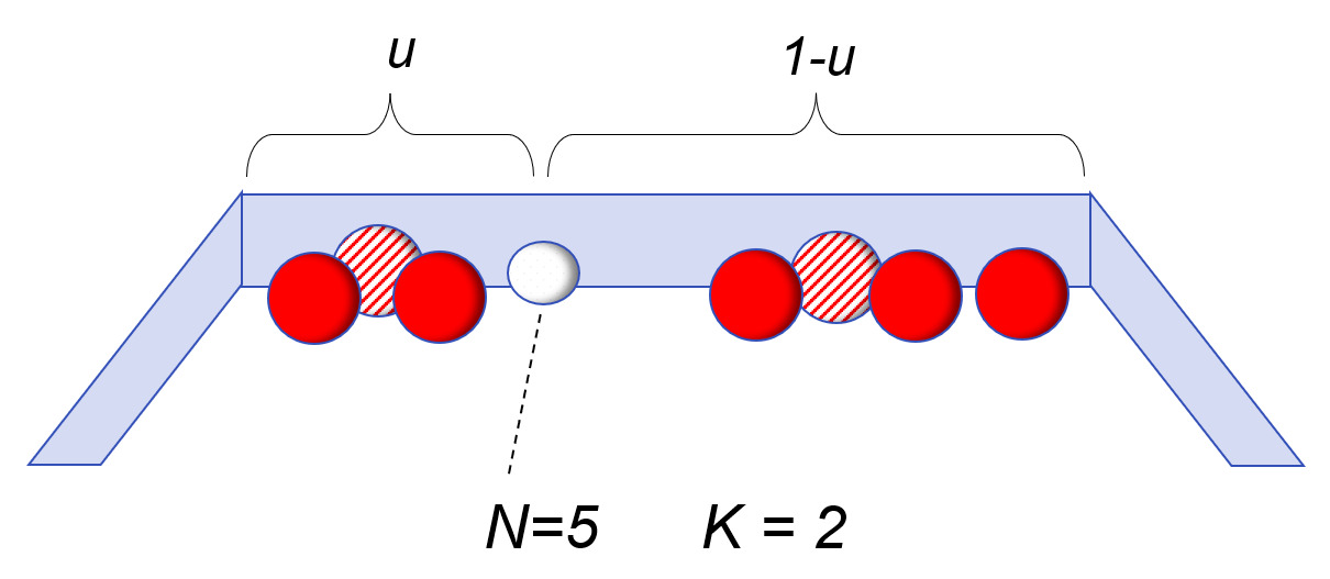
The expression for the posterior expected value can also be written in the familiar credibility form:

\[\begin{array}{c} E\left( u|P,Q \right) = \frac{P}{P + Q} \cdot \left( \frac{N}{N + K} \right) + \frac{1}{2} \cdot \left( \frac{K}{N + K} \right)\\ \\ N = P + Q,\ K = 2 \end{array}\tag{2.1.4}\]

In the credibility form, \(N\) is the number of actual balls observed, and \(K\) is the number of “imaginary” balls representing the prior knowledge.

Though Richard Price talked about the usefulness of this when the number of actual observations was small on either the left or right, there are similarities to problems faced in insurance. For example, in pricing excess-of-loss insurance or reinsurance, there are often problems of “free cover.” This arises when no losses in the available historical experience exceed some threshold; we might hear “there has never been a loss greater than $10,000,000.” To account for this “free cover” problem, the actuary or underwriter may add an imagined loss to the history based on an estimated return period: for example, to assume we have one very large loss every 20 years.

2.2. Ridge Regression

The method of Ridge Regression was introduced in a paper by Hoerl and Kennard (1970), but the method has expanded to be one of the building blocks of regularization, sometimes called the “secret sauce” of machine learning.^[3] The expansion to data augmentation was introduced in Allen (1974).

The key insight of the paper is that when a regression model has many parameters relative to the number of data points, and especially if some predictors are correlated (i.e., “nonorthogonal”), the predictive value of the model can be improved by introducing some bias in the parameter estimates. The bias is introduced as “shrinkage” such that regression coefficients are shrunk towards zero compared to the estimates derived by ordinary least squares.

The estimated regression coefficients in Ridge Regression are found using formula (2.2.1). An amount \(k\) is added to each element on the diagonal of the square matrix \(\left( X^{T} \cdot X \right)\). This stabilizes the calculation compared to the ordinary least squares (OLS) estimate when \(k = 0\).

\[\widehat{\beta} = \left( X^{T} \cdot X + k \cdot I \right)^{- 1} \cdot X^{T} \cdot Y \tag{2.2.1}\]

Hoerl & Kennard also note that Ridge Regression can be viewed as a Bayesian model.

“Viewed in this context, each ridge estimate can be considered as the posterior mean based on giving the regression coefficients, \(\beta\), a prior normal distribution with mean zero and variance-covariance matrix \(\Sigma = \left( \delta_{i},\delta^{2}/k \right)\). For those that do not like the philosophical implications of assuming \(\beta\) to be a random variable, all this is equivalent to constrained estimation by a nonuniform weighting on the values of \(\beta\).”

Not surprisingly, this means that the ridge estimate of the model coefficients can be expressed as a linear average of the OLS estimate with the complement of zero. The credibility weight, \(Z\), is a matrix, equivalent to the multidimensional Bühlmann-Straub formula. Miller (2015) gives a more complete description of the connection between ridge regression and credibility.

\[\begin{aligned} {\widehat{\beta}}_{ridge} &= Z \cdot {\widehat{\beta}}_{OLS} + (I - Z) \cdot 0\\ where\ Z &= \left( X^{T} \cdot X + k \cdot I \right)^{- 1} \cdot \left( X^{T} \cdot X \right) \end{aligned}\tag{2.2.2}\]

Ridge regression is usually presented using a squared error loss function (sum of squares) plus a penalty term on the magnitude of the fitted coefficients. For a given value of \(k\), the ridge estimate is equivalent to minimizing this penalized sum of squares.

\[\begin{aligned} Penalized\ Sum\ of\ Squares &= \sum_{i = 1}^{n}\left( y_{i} - {\widehat{y}}_{i} \right)^{2}\\ & \quad + k \cdot \sum_{j = 1}^{p}\beta_{j}^{2} \end{aligned}\tag{2.2.3}\]

Alternative derivation of the ridge formula is to augment our observed data with an additional row for each parameter.:

\[\begin{bmatrix}Y \\0\end{bmatrix} = \begin{bmatrix}X \\\sqrt{k} \cdot I\end{bmatrix} \cdot \beta + \varepsilon \tag{2.2.4}\]

Draper and Smith (1998) refer to this not as “data augmentation” but as “the phony data viewpoint .” That characterization may help explain some of the reluctance to talking about this augmentation form: who would want to be accused of publishing a scientific paper that made use of “phoney” data?

Rather than the matrix format, we can also think of this as a weighted regression. In this case, we could simulate a very large number of points from a “prior” distribution with zero slope. The simulated points are then downweighted so that they get a total weight as though there were K representative points. For example, we simulate M=10,000 random points and then assign them each a weight of K/M.

This can be illustrated in the case of a simple linear regression with only one predictor. In this graph the large blue points represent our actual observed data points. The scatter of small red points represents simulated data (with slope =0), and the small size of these points represents the fact that they are downweighted. The red points play the same role in Ridge Regression that the “imaginary balls” played in Bayes’ thought experiment.

Figure 2.1.Ridge Regression

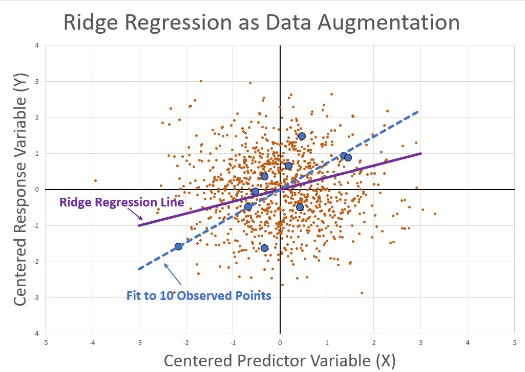
Performing a weighted regression on the augmented data set (actual data plus the downweighted simulated data) will result in exactly the same result as ridge regression for a sufficiently large simulation.

Of course, in the simple case, where we have a linear model and a squared error loss function, there is no need to perform the simulation. It is only useful as a way of understanding what the ridge regression is doing. However, if we move to more complex non-linear models or alternative loss functions, then the closed-form ridge regression does not work but the simulation could still be applied.

The main advantage in viewing ridge regression as data augmentation rather than the penalized regression form (2.2.3) is that the smoothing parameter takes on a physical meaning. It represents how many pseudo-data points are added to the actual data.

2.3. Generalized Linear Models (GLM)

The insight behind Generalized Linear Models (GLM) is that a family of statistical models (logistic regression, linear regression, and Poisson regression) can all be unified in a single theoretical model. This was introduced in Nelder and Wedderburn (1972) and generalized further in Wedderburn (1974) to include quasi-likelihood. The model is very flexible and powerful and has been extended in many ways since it was originally introduced.

In Property & Casualty insurance, GLM is used as a central tool for ratemaking. Credibility can be included effortlessly in this application.

GLM includes, as special cases, members of the natural exponential family. This is the same family of distributions described by Jewell (1974) when discussing credibility means from the Bayesian perspective. This subset of GLMs have conjugate priors that allow for credibility to be implemented as weighted averages.

Gelman et al. (2013) summarize this advantage for the conjugate families as follows (Section 16.2, page 409).:

A sometimes helpful approach to specifying prior information about \(\beta\) is in terms of hypothetical data obtained under the same model, that is, a vector \(y_{0}\), of \(n_{0}\) hypothetical data points and a corresponding \(n_{0}\ \times k\) matrix of explanatory variables, \(X_{0}\). …the resulting posterior distribution is identical to that from an augmented data vector \(\begin{pmatrix} y \\ y_{0} \end{pmatrix}\) – that is, \(y\) and \(y_{0}\) strung together as a vector, not the combinatorial coefficient – with matrix of explanatory variables \(\begin{pmatrix} X \\ X_{0} \end{pmatrix}\) and a noninformative uniform prior density on \(\beta\). For computation with conjugate prior distributions, one can thus use the same iterative methods as for noninformative prior distributions.

The GLM application is therefore a generalization of Ridge Regression.

Use of data augmentation in GLM is also described in past literature in Bedrick, Christensen, and Johnson (1996), Huang et al. (2020) and Greenland (2006, 2007). Greenland describes the process as:

"Expressing the prior as equivalent data leads to a general method for doing Bayesian and semi-Bayes analyses with frequentist [e.g., GLM] software:

(i) Construct data equivalent to the prior, then.

(ii) Add those prior data to the actual study data as a distinct (prior) stratum."

Greenland goes on to note that data augmentation is not limited to conjugate cases; in fact, any prior assumption can be converted to an equivalent data representation. He argues that “to say a given prior could not be viewed as augmenting data means that one could not envision a series of studies that would lead to the prior.”

Similar to the ridge regression example, regularization in GLM can be implemented either as a penalty term or as data augmentation. The data augmentation approach has a number of advantages:

1. Data augmentation gives a clear meaning to how much the “prior” information is allowed to influence the result. The smoothing parameter in penalized regression is harder to interpret.

2. Data augmentation allows the GLM software to use the very efficient Iteratively Reweighted Least Squares (IRLS) algorithm to estimate the model parameters.

3. Data augmentation does not require predictor variables to be centered or standardized.

4. Data augmentation allows the model to regularize towards an informative prior (e.g., an expiring rating plan) rather than naively to an overall average loss cost.

We proceed to the key question of the source of the prior data used to augment the observed data. There are two basic philosophies:

Empirical Bayes

• “Let the data speak for itself.”

• Complement of credibility is some summary of the data itself (e.g., overall average loss cost)

• Credibility weight is determined from the data (e.g., via cross validation)

Subjective Bayes

• “Borrow strength from other relevant information.”

• Complement of credibility is from some other data source (e.g., expiring rating plan, industry or peer company data, expert judgment, etc.)

• Credibility standard is assigned by the analyst based, in part, on the reliability of the external data source

The “subjective” label may be a misnomer because the prior can be taken from an existing rating plan or other objective data.

We can illustrate the difference with a small numerical example from motorcycle crash frequencies. The data comes from Sweden,^[4] but can illustrate the idea more generally. The top section is a summary from the actual data, showing the exposure units on the left, historical count in the middle, and frequency (counts per exposure) on the right. The bottom section is the “prior” data that is used to augment the actual observed experience.

An example of Empirical Bayes implementation is in the chart below. The “prior” frequency is calculated as a constant value, 1.05%, equal to the average of the actual data across all rating classes. In practice, we do not need to use just a single number but the “prior” can be any simpler model using the observed data.

Figure 3.1.GLM with “Empirical Bayes”

The alternative to the Empirical Bayes approach is Subjective Bayes. If the prior data has been taken from a relevant data source, then it is considered an 'informative" prior and given more prior weight than in the Empirical Bayes example. The weight in the table below is increased from 10 exposures per rating class to 100.

In practice, it is useful to include a control variable to identify records from the original observed data from the “prior” data. This allows the model results to balance back to the observed data and only use the prior data to adjust relativities between classes. Greenland (Part 2, page 199) says, “One also adds a new regressor to the model to indicate whether a record is from the X-prior or from the actual data. If we call this indicator ‘Prior’, we set Prior=1 for the… prior records and Prior=0 for the actual data.”

Figure 3.2.GLM with “Subjective Bayes”

The choice between the Empirical and Subjective approaches will depend upon the data sources available and the purpose of using the augmented data. If we are only trying to keep the model from over-fitting to noisy data, then using Empirical Bayes to regularize the model may be sufficient. If we are trying to limit the disruption in charged premium in a revised rating plan, then regularizing towards the old model may be a better choice.

3. Insurance example: size-of-loss curve-fitting

The examples in section 2 of this paper are well known in the Statistical literature. The size-of-loss example may be less known but is simply another application of the same concept.

3.1. Pareto Example

We begin by defining the cumulative distribution function (CDF) for the single parameter Pareto distribution.

\[F(y) = {1 - \left( \frac{T}{y} \right)}^{\alpha}\ \ \ y \geq T \tag{3.1.1}\]

The distribution is defined for loss amounts greater than some “threshold” value, \(T\).

The MLE estimate for the shape parameter is given by:

\[{\widehat{\alpha}}_{MLE}^{- 1} = \frac{1}{N}\sum_{i = 1}^{N}{\ln\left( \frac{y_{i}}{T} \right)} \tag{3.1.2}\]

The case where a policy limit cap may apply to some of the large losses is a small modification, as shown below, where \(C\) represents the number of losses that hit their policy limit (i.e., how many loss amounts are “censored”).

\[{\widehat{\alpha}}_{MLE}^{- 1} = \frac{1}{N - C}\sum_{i = 1}^{N}{\ln\left( \frac{MIN\left( y_{i},{PL}_{i} \right)}{T} \right)} \tag{3.1.3}\]

Because the Pareto distribution is a member of the exponential family,^[5] we can also find a conjugate prior.^[6] If we assume that the shape parameter, \(\alpha\), has a prior Gamma distribution, with a shape parameter \(K\), then the credibility can be done with simple weighted averages.

\[g(\alpha) = \frac{\alpha^{K - 1}}{b^{K} \cdot \Gamma(K)} \cdot exp\left( - \frac{\alpha}{b} \right)\ \ \ E(\alpha) = b \cdot K \tag{3.1.4}\]

With this conjugate relationship, the posterior mean can be written in a simple form, consistent with the Bühlmann-Straub theory.

\[\frac{N + K}{E\left( \alpha|\left\{ y_{i} \right\}_{i = 1}^{N} \right)} = \frac{N}{{\widehat{\alpha}}_{MLE}} + \frac{K}{E(\alpha)} \tag{3.1.5}\]

The mean for the posterior distribution of \(\alpha\) can be found directly given the MLE estimate from the data, plus the mean and standard deviation of the prior distribution. Alternatively, we can re-write this expression as:

\[\begin{aligned} \frac{N + K}{E\left( \alpha|\left\{ y_{i} \right\}_{i = 1}^{N} \right)} &= \sum_{i = 1}^{N}{\ln\left( \frac{y_{i}}{T} \right)} + K\\ & \quad \cdot \left( \frac{1}{M} \cdot \sum_{i = 1}^{M}{\ln\left( \frac{y_{i}^{(0)}}{T} \right)} \right) \end{aligned}\tag{3.1.6}\]

In this alternative form, we draw a large number, \(M\), of simulated losses \(y_{i}^{(0)}\) from the prior predictive distribution and include these as part of an augmented data set. The “trick” here is that each simulated pseudo-data point is downweighted by a factor of \(K/M\).

We see then that there are two equivalent credibility methods that can be applied.

1. Fit Pareto via MLE to the observed data and then credibility weight the estimated parameter with a benchmark parameter as a complement.

2. Augment the observed data with simulated data drawn from the prior information and perform MLE on the augmented data set.

The first method is clearly easier when we have a one-parameter curve with a conjugate prior. The data augmentation method is more useful when more complex curves are needed.

For the Pareto case, when we also assume a conjugate prior Gamma distribution on the single shape parameter, the simulation of augmented data is not needed. We can simply use formula (3.1.5) directly. But the data augmentation approach proves much more useful for other curves.

3.2. Extensions to Other Curves

The use of data augmentation can be used directly in MLE curve-fitting so long as we have a “prior” benchmark size-of-loss curve to use.

We can illustrate this with the “mixed exponential” curve used by the Insurance Services Office (ISO). The curve form – as the name implies – is a discrete mixture of exponential distributions. Typically the number of curves in the mix is between eight and twelve, which is sufficient to approximate a wide range of loss sizes.

The exponential distribution is easy to simulate from, and the weighting factors \(w_{j}\) allows for stratified sampling to make the calculations very efficient.

\[F(y) = \sum_{j = 1}^{W}{w_{j} \cdot \left( 1 - exp\left( - \frac{y}{\mu_{j}} \right) \right)}\ \ \ \ 1 = \sum_{j = 1}^{W}w_{j} \tag{3.2.1}\]

We can simulate some large amount, \(M\), from each of the exponential curves. In the loglikelihood calculation, the downweighting adjustment for each point is then \(w_{j} \cdot K/M\) rather than just \(K/M\).

The MLE for whatever size-of-loss curve form is selected (e.g., lognormal, Burr, Pareto, etc.) is performed on the augmented data set, including the downweighting for the simulated pseudo-data.

As with the GLM example, there is great flexibility in the choice of prior information.

Perhaps we do not have a benchmark severity curve in the form of a mixed exponential. Instead, we have loss data for a group of “peer” companies.^[7] For example, an insurance company may specialize in writing Trucking risks, and has gathered historical loss data for, say, five Trucking companies. If a severity curve is needed for the pricing of one of these companies, we can still use the losses from the other four companies in the curve fit, but with reduced weights so that they do not overly influence the fit for the company being priced.

4. CONCLUSIONS

The idea of data augmentation has a long history in Statistics and can be derived either from Classical (Frequentist) or Bayesian frameworks. In the Bayesian theory, it is an exact solution for conjugate distributions in the exponential family.

For insurance applications, data augmentation is a useful way of interpreting credibility models, because it shows explicitly how we can “borrow strength” by blending in data from multiple sources.

This paper shares some examples as a way of understanding this interpretation of credibility and hopes to spur more research for practical applications. Applications in GLM look to benefit most from such methods.

Acknowledgment

The author gratefully acknowledges the helpful comments from Avraham Adler, Jonathan Hayes, Max Martinelli, Ulrich Riegel, Ira Robbin, and Janet Wesner. All errors in the paper are solely the responsibility of the author.

Abbreviations used in the paper

Biography of the Author

David R Clark, FCAS is a senior actuary with Munich Re America Services, working in the Pricing and Underwriting area. He is a frequent contributor to CAS seminars and call paper programs.