Claim Counts Prediction Using Individual Data with ReSurv

1. Introduction

In the non-life insurance practice, the term reserves is used to indicate the insurer’s estimate of unpaid claims that were incurred prior to the financial statement reporting date (Friedland 2010, 13). One part of the reserve includes the so-called Incurred But Not Reported (IBNR) claims. Since the number and average size of IBNR claims are not known at the time the reserve is computed, actuaries must estimate them. One option is to model the number and size of IBNR claims separately. In this paper we present a method for estimating the number of claims. While not being discussed here further, one simple way of estimating the average size of IBNR claims is to take the average of the severity of historical claims, possibly dependent on the reporting delay and further claim features, $x$. In future work we will look into ways to handle frequency and severity together.

Modelling of future reported claim counts usually utilises development triangles, an aggregate representation of the reserving data that is standard practice in the industry (Brown, Julga, and Merz 2023). A development triangle is a set of observations

$$\mathcal{O}=\left\{O_{k j}: k, j=0, \ldots, m ; k+j \leq m\right\}, \quad m>0,$$

where $O_{k j}$ is the total number of reported claims in accident date $k$ with reporting delay $j$; i.e., the claim has been reported in $k+j$. Here, $k=0$ denotes the earliest accident date and $m>0$ is the input dimension of the development triangle. A commonly used model to calculate reserves from development triangles is the chain-ladder. Given the cumulative triangle

$$\begin{aligned} C_{kj}= \sum_{l\leq j} O_{kl}, \quad k, j=0, \ldots, m ; k+j \leq m, \end{aligned}\tag{1}$$

one calculates so-called age-to-age factors $\tilde f_{kj}$,

$$\begin{aligned} \tilde f_{k j}&=C_{kj} / C_{k,{j-1}}, \quad k=0,\dots,m; j=1,\dots,m; j+k\leq m. \end{aligned}\tag{2}$$

These age-to-age factors cannot be directly used for prediction since they are only defined on the upper triangle $j+k\leq m$. Instead, they are averaged over accident dates $k$:

$$\hat f_{j}= \sum_{k=0}^{m-j} w_k \tilde f_{kj} \tag{development factors}.$$

Various ways of averaging can be used, but the most common is the volume-weighted average $w_k=C_{k ,j-1}/{\sum_{l=0}^{m-j} C_{l,j-1}}$. Lastly, future reported claims are derived via:

$$\widehat C_{kj}= \begin{cases} \widehat{f}_{j} C_{k,j-1} & \text{for}\ k+j=m+1,\\ \widehat{f}_{j} \widehat C_{k,j-1}& \text{for}\ k+j>m+1. \end{cases}$$

While reserving models for aggregate data have a long history in the industry, the advent of new advanced computing tools has encouraged actuarial professionals to explore reserving models based on individual data (Richman 2021). Often the more advanced techniques are based on sound theory, but there is no open-source implementation that makes the models directly applicable in practice. A notable exception is the hierarchical model in Crevecoeur et al. (2023), implemented in the R package hirem (Crevecoeur and Robben 2024). In this manuscript we present a pipeline for individual claims reserving using the R package ReSurv. Our package calculates accident date and feature-dependent development factors that can be used to predict future IBNR claims. Indeed, instead of chain-ladder’s development factors $\hat f_j$, the ReSurv package calculates development factors

$$\begin{aligned} \hat f_{kj}(x), \quad k=0,\dots,m;j=1,\dots,m \end{aligned}\tag{3}$$

that may additionally depend on accident date $k$ and some features $x$. It is important to note here that the development factors the ReSurv packages derives are defined on the whole square including the lower triangle, $k+j>m$, and can therefore be directly used for prediction. This is different to the age-to-age factors that are only defined on the upper triangle $k+j\leq m$, cf. equation (2). The features $x$ can be seen as reflecting different development triangles (e.g., business line, cover type or claim type) which the ReSurv package can handle simultaneously. For example, one could consider one feature $x=$ claim_type that can take either value PD for Property Damage claims or BI for Bodily Injury claims. In this case we would have two triangles:

$$\small{ O(\mathrm{PD})=\left\{O_{k j}(\mathrm{PD}): k, j=0, \ldots, m ; k+j \leqslant m ; \text { clain_type }=\mathrm{PD}\right\} . }$$

$$\small{ \mathcal{O}(\mathrm{BI})=\left\{O_{k j}(\mathrm{BI}): k, j=0, \ldots, m ; k+j \leqslant m ; \text { claim_type }=\mathrm{BI}\right\}, \quad m>0 }$$

Given multiple cumulative triangles $C_{kj}(x)$, prediction is now done via

$$\hat{C}_{k j}(x)= \begin{cases}\hat{f}_{k j}(x) C_{k, j-1}(x) & \text { for } k+j=m+1 \\ \hat{f}_{k j}(x) \hat{C}_{k, j-1}(x) & \text { for } k+j>m+1\end{cases} \tag{4}$$

Lastly, for reporting purposes one usually wishes to have an aggregation in, e.g., quarters or years. However, the original input $j,k$ for the ReSurv package is assumed to be as granular as possible and may, e.g., be in days. To this end the ReSurv allows to specify an output dimension $M$ as a multiple of the input dimension ($(m \mod M) = 0, M < m$). On the output scale $M$, we will work with a $j^\prime, k^\prime = 0,\ldots,M$ and we will have the cumulative triangle

$$C_{k^{\prime} j^{\prime}}^{\prime}(x)=\sum_{h, \nu=0, \ldots, m:\left\lfloor h \cdot \frac{M}{m}\right\rfloor \leqslant k^{\prime} ;\left\lfloor\nu \cdot \frac{M}{m}\right\rfloor \leqslant j^{\prime}} O_{h \nu}(x) .$$

The ReSurv package also calculates feature-dependent development factors for the output granularity $M$:

$$\hat{f}_{k^{\prime} j^{\prime}}^{\prime}(x), \quad k^{\prime}=0, \ldots, M ; j^{\prime}=1, \ldots, M,$$

with

$$\widehat{C}_{k^{\prime} j^{\prime}}^{\prime}(x)= \begin{cases}\hat{f}_{k^{\prime} j^{\prime}}^{\prime}(x) C_{k^{\prime} j^{\prime}-1}^{\prime}(x) & \text { for } k^{\prime}+j^{\prime}=M+1, \\ \hat{f}_{k^{\prime} j^{\prime}}^{\prime}(x) \widehat{C}_{k^{\prime} j^{\prime}-1}(x) & \text { for } k^{\prime}+j^{\prime}>M+1 .\end{cases} \tag{5}$$

The rest of the paper is organized as follows. In Section 1.1, we give a short overview on the machine learning methods employed and where to find further reading. In Section 1.2, we provide a simplified explanation of the methodology in Hiabu, Hofman, and Pittarello (2023); for a full review, please refer to the main manuscript. After describing in detail how to install the package, we discuss a pipeline for individual reserving in Section 2. We show a data application on a simulated data set in Section 3.

1.1. Machine learning foundation

ReSurv leverages three machine learning techniques in its implementation: splines, feed-forward neural networks and gradient boosting. While familiarity with machine learning principles can enhance usability and help with modelling decisions, the interpretability of the results remains independent of the user’s expertise in this area. Our package is designed to provide meaningful results regardless of the user’s background in machine learning. For readers interested in an introduction to machine learning, we refer to Section 7 of James et al. (2023) for a gentle introduction to splines and to Section 10.2 in James et al. (2023) for an accessible introduction to feed-forward neural networks. Section 10.7 provides an overview of the optimisation task and the algorithm used to minimise the objective functions. Section 10 in Géron (2019) provides a less mathematical introduction to neural networks with accompanying Python code. For further reading, Goodfellow, Bengio, and Courville (2016) is a comprehensive handbook on neural networks. Sections 8.1 and 8.2 in James et al. (2023) will give a better understanding of tree-based methods, while Chen and Guestrin (2016) introduce and explain the gradient boosting algorithm.

1.2. Hiabu, Hofman, and Pittarello 2023 in a nutshell

The mathematical basis for ReSurv follows from the formulation of the reserving problem in a survival analysis setting. We model the reporting delay of individual claims by specifying a regression model for the corresponding hazard function. Consider a set of reported claims. Each observed claim $i$ is associated with an accident date $u_i$, a reporting delay from accident $t_i$, and $p$ covariates $x_i \in \mathbb{R}^p$ that can be categorical or numerical. We specify the following regression model for the hazard function

$$\begin{align} \alpha(t|u,x) &= \lim_{h \downarrow 0} P \left\{t_i \in [t, t+h)|t_i \geq t , u_i=u, x_i= x\right\}\\&=\alpha_0(t)e^{\phi \left( x, u \right)}, \end{align} \tag{6}$$

where $\alpha_0(t)$ is called the baseline hazard and $e^{\phi \left( x, u \right)}$ is the risk score; a component that depends on the features ${x}_i$, and the accident date $u_i$. Note that the hazard function is defined in its own right as infinitesimal conditional probability. In particular it is not defined via the intensity of a stochastic process. The main use of the hazard function in the ReSurv package after estimating it is its transformation into development factors via equation 8 described below. In that sense the hazard function can be seen as intermediate object used in the reserving task. Actuaries reading this manuscript will likely be familiar with the concept of GLM regression for modelling frequencies in insurance pricing. In pricing, one assumes that the number of claims $Y_i$ is Poisson distributed conditionally on some covariates $X_i$ and an exposure $W_i$

$$Y_i|W_i,X_i \sim \text{Poisson}\left(W_i \exp\left(\theta^T_{\text{GLM}}X_i\right)\right). \tag{7}$$

In this case, it is possible to derive an analytic solution for an estimator of the parameter $\theta_{\text{GLM}}$ by minimising the model negative likelihood. In this manuscript, we perform regression on reserving data using the survival model in equation 6. In our application we look for an estimate of the risk score $e^{\phi \left( x, u\right)}$ and the baseline $\alpha_0(t)$. For a detailed comparison of hazard modelling and Poisson regression, we refer the reader to Carstensen and Diabetes (2004). It is important to note that, unlike the pricing case discussed therein, our approach does not rely on a distributional assumption and the hazard function estimation relies on the partial-likelihood theory described in Hiabu, Hofman, and Pittarello (2023). Lastly, depending on the machine learning model that we choose, the risk score will have a different specification. Estimation of $\phi \left( x, u\right)$ can be performed in ReSurv with three different algorithms: the Cox model (COX, Cox 1972), neural networks (NN, Katzman et al. 2018) and gradient boosting (XGB, Chen and Guestrin 2016).

• In Cox (1972), the logarithm of the risk score function is assumed to be linear, $\phi \left( x, u\right)=\theta^T x + \theta_u u$, with $\theta \in \mathbb{R}^p$ and $\theta_u \in \mathbb{R}$. Our package provides the option to include splines for modelling continuous features.

• In NN, $\phi \left( x, u\right)$ is a feed-forward neural network.

• In XGB, $\phi \left( x, u\right)$ is an ensemble of decision trees, i.e., functions that are piecewise constant on rectangles.

After an estimator $\hat \phi \left( x, u \right)$ is derived, the baselines $\alpha_0(t)$ is estimated using the full-likelihood where it is assumed that claim reports are uniformly distributed within a tie. Putting the estimators together we derive an estimator of the hazard function

$$\hat \alpha(t|u,x) = \hat \alpha_0(t)e^{\hat\phi \left( x, u \right)},$$

Finally, we model the development factor from reporting delay $j-1$ to $j$ and accident date $k$ as

$$\tilde {f}_{kj}(x) = \frac{2+ \hat \alpha(j|k,x) }{2- \hat \alpha(j|k,x)}. \tag{8}$$

For a derivation and discussion of formula (8), we refer to Pittarello (2024), but remark for those familiar with mortality life tables (Chiang 1972) that formula (8) is analog to transforming the central mortality rate into conditional probabilities of dying. From here, these development factors can be applied using the chain-ladder rule for forecasting, cf., equation (4). By introducing feature and accident date dependency in the hazard estimation, we allow the same properties in the development factors.

Installation

The ReSurv package can be installed from The Comprehensive R Archive Network (CRAN).

>>> install.packages("ReSurv")

The developer version of ReSurv can be installed from GitHub.

>>> library(devtools)
>>> devtools::install_github("edhofman/resurv")

The package can then be imported in R using the command

>>> library(ReSurv)

Additional resources on our project can be found at https://github.com/edhofman/ReSurv. We remark that this manuscript refers to version 1.0.0 of our package:

>>> packageVersion("ReSurv")
    1.0.0

The main page of the help guide of our package can be accessed with the following command:

>>> help(package="ReSurv")

1.3. Handling the Python dependency

In this Section we illustrate the approach we use to handle the Python dependency in our package. The ReSurv package interfaces with a Python implementation to implement the NN models. The reader who is not interested in using the NN models can disregard this Section. The interaction with Python is handled by creating an isolated virtual environment through the install_pyresurv function

>>> install_pyresurv()

The default name of the virtual environment is "pyresurv".

We then suggest refreshing the R session and to import the ReSurv package in R using

>>> library(ReSurv)
>>> reticulate::use_virtualenv("pyresurv")

This approach uses the reticulate package implementation for interfacing R and Python (Ushey, Allaire, and Tang 2024).

Managing Multiple Package Dependencies

In case the user is working with other libraries that use isolated package specific environments, the most straightforward solution would be installing a dedicated environment for both. Below, an example using the R package pysparklyr.

>>> envname <- "./venv"
>>> ReSurv::install_pyresurv(envname = envname)
>>> pysparklyr::install_pyspark(envname = envname)

The interested reader can read more about this topic in the vignette Managing an R Package’s Python Dependencies.

2. IBNR modelling using ReSurv

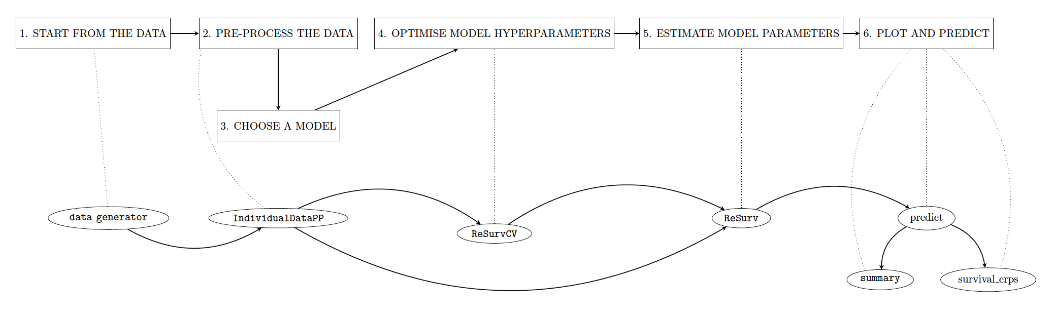
In this section, we illustrate individual claims reserving in six steps that an actuary can take to perform individual reserving using our software.

2.1. A pipeline for modelling expected counts

1. Start from the data. In Section 2.2, we discuss the required structure of the input data. In Section 2.2.1 we will use the simulator embedded in our package to generate a synthetic reserving data set to show the usage of ReSurv.

2. Pre-process the data. Before using a reserving model, individual data must be elaborated in a format that is ready for using the individual model. This is done in Section 2.3.

3. Choose a model. As mentioned earlier, our package allows us to model the log-risk function using three different models (COX, NN and XGB). The aim of Section 3 is to compare the three available approaches’ performance according to some performance metrics that we will define.

4. Optimise the model hyperparameters. After a brief introduction on hyperparameters in machine learning, the objective of Section 2.4 is to describe hyperparameters tuning. Section 2.5 explains how Bayesian hyperparameter tuning can be performed utilizing the ParBayesianOptimization package.

5. Estimate the model parameters. Once we have estimated the hyperparameters of the models, we can fit our models using the ReSurv method, as described in Section 2.6.

6. Visualize claim development and predict IBNR. The optimised model can be used to plot feature-dependent development factors as well as predict IBNR claims for different data granularities. For example, if actuaries have daily data available for fitting, our approach is flexible enough to report and visualize future claims on a monthly, quarterly or annual scale. This is shown in Section 2.7.

Figure 1.At the bottom, we show the six steps of individual reserving illustrated in Section 2. The steps are numbered and connected by solid arrows. The six steps can be performed using the ReSurv package tools that we show in the upper part of the figure. The package tools we are showing are described in detail in Section 3. Each package tool is linked to the corresponding step by a dotted arrow. The directional arrows in the diagram indicate the flow of information or processes, where the output of one step serves as the input for the next.

2.2. How should my input data look?

We begin this Section considering the least number of columns that should be included in the input data:

• Accident date of the claim, $k$ (in calendar time).

• Reporting date of the claim, $k+j$ (in calendar time).

As we will show in the next two examples, the input dates can be either in Date or numeric format.

Optionally, the data can also include a set of static covariates, categorical and/or continuous, that can be used for modelling the feature-dependent development factors, $x$, in equation 3.

The individual input data can be of two types. The first option is working with a data set where each row corresponds to a claim. An example is the data that we will simulate in Section 2.2.1. The first ten records of our simulated data are shown in Table 1. The data set contains one categorical feature $x=$claim_type and the relevant dates: accident date ($k$=AP) and reporting date ($k+j$=RP). In this example, AP and RP are in Date format.

Alternatively, in the input data there could be multiple records for each claim. As an example, we consider the data set test_transaction_dataset, part of the SynthETIC package. The data set is displayed in Table 2. test_transaction_dataset is the case of an individual reserving data set where multiple events for each individual are recorded (e.g., multiple payments) and each individual is associated with a unique identifier (claim_no). In this example, the reporting date (RP) and the accident date (AP) are in numeric format.

Since the objective of the ReSurv package is modeling the reporting delay which we assume unique for each individual claim, these multiple records will not be part of our modeling but the preprocessing of this type of input can be performed internally by our software.

2.2.1. Data simulation

In this Section, we generate a synthetic data set to show the usage of the ReSurv package. This section may be ignored by a reader who already has a data set in the input format described in Section 2.2.

Let us consider the data$\_$generator function.

>>> input_data <- data_generator(random_seed = 7,
                             scenario = "alpha",
                             time_unit = 1 / 360,
                             years = 4,
                             period_exposure = 200)

This function contains $5$ different parameters:

• The random$\_$seed, integer. It guarantees full replicable code.

• Our package offers $5$ different simulated scenarios that can be used to replicate our manuscript analysis. The scenarios are described below and selected with the parameter scenario. Here, we choose to simulate from the so-called scenario Alpha. The user can input one of the following character: ’alpha’, ’beta’, ’gamma’, ’delta’, ’epsilon’.

• time_unit, numeric. It controls the data granularity (time unit) as a fraction of a calendar-year. In our manuscript we generate daily data and set time_unit$=1/360$. Implicitly, we are assuming that a year is made of 360 days.

• years, integer. This is the total number of accident years in the simulation. In the manuscript we use a four calendar year time horizon for daily data.

• The period_exposure consists of the total underwriting volume for time unit. In our manuscript we have a daily volume of $200$ contracts.

Our package allows to simulate reserving data under $5$ scenarios using the function data$\_$generator. The simulator is based on the SynthETIC package (Avanzi et al. 2021). We named the $5$ scenarios Alpha, Beta, Gamma, Delta, Epsilon. The $5$ scenarios contain the information described in Table 3. Our simulated data consist of a mix of short tail claims (claim_type 0) and claims with longer time to report (claim_type 1). We chose the parameter of the simulator to resemble a mix of property damage (PD, claim_type 0) and bodily injury (BI, claim_type 1).

However, each scenario has distinctive characteristics. Scenario Alpha is a mix of claim_type 0 and claim_type 1 with the proportion of type 0 and 1 claims held constant across the accident days. Chain-ladder is expected to work well in this case such that we cannot expect ReSurv to provide improved prediction performance. In scenario Beta the proportion of claim_type 1 claims are decreasing in the most recent accident dates. In scenario Gamma we add an interaction between claim_type 1 and accident date: in a real world setting this can be motivated by a change in consumer behavior or company policies resulting in different reporting patterns over time. In scenario Delta, we introduce a seasonality effect period (spring, summer, winter, fall) dependent on the accident date for the proportion of claim_type 0 versus claim_type 1. In the real world, the scenario Delta resembles seasonal changes in the portfolio composition. Chain-ladder is expected to have problems handling scenarios Beta, Gamma and Delta accurately, and the ReSurv package is expected to provide significantly better predictions in those cases. In Scenario Epsilon, Chain-ladder is expected to have better predictive performance than our models because we violate our model assumptions by assuming an effect of claim_type and AD on the baseline. The object input_data is a data.frame frame (each row is a claim observation with data elements attached) and its structure can be displayed with the following command.

>>> str(input_data)
    'data.frame':   29088 obs. of  4 variables:
     $ claim_number: int  1 2 3 4 5 6 7 8 9 10 ...
     $ claim_type  : num  0 0 0 0 0 0 0 0 0 0 ...
     $ AP          : num  1 1 1 1 1 1 1 1 1 1 ...
     $ RP          : num  19 201 895 883 36 ...

We show the empirical cumulative density function of the simulated notification delay (Figure 2a) and the data distribution by claim type (Figure 2b). We can notice quicker notification for claim_type 0. The two claim types have similar volumes at run-off (ultimate claims).

Figure 2.Empirical simulated cumulative distribution function (left-hand side) and data distribution by claim type (right-hand side).

2.3. Data pre-processing

Before fitting our model on the data, the individual data must be pre-processed. In our software, this can be achieved with the built-in function IndividualDataPP. This step involves the dummy encoding of categorical features using the function dummy_cols from the fastDummies package (Kaplan 2020) and scaling of continuous features using the MinMax Scaler approach (Wüthrich 2018). Dummy encoding is used to convert categorical variables into numerical format. It creates separate columns for each category (or level) of the variable, assigns a 1 if the observation belongs to that category and a 0 if it does not. MinMax scaling is a normalization technique that transforms data to a specific range, typically [-1, 1]. In the MinMax Scaler approach, we consider a continuous covariate $x^\nu_i$ with $x_i=\left(x^1_i, \ldots, x^\nu_i, \dots, x^p_i\right)$ and apply the transformation

$$x^\nu_i \mapsto \bar x^\nu_i: \bar x^\nu_i=2 (x^\nu_i- \min(x^\nu_i))/(\max(x^\nu_i)- \min(x^\nu_i))-1,$$

to bring all features to a comparable scale.

IndividualDataPP creates an individual data set that is ready to be modelled.

>>> individual_data <- IndividualDataPP(data = input_data,
                                    categorical_features = "claim_type",
                                    continuous_features = "AP",
                                    accident_period = "AP",
                                    calendar_period = "RP",
                                    input_time_granularity = "days",
                                    output_time_granularity = "quarters",
                                    years = 4)

• The input data. E.g., the simulated output of data$\_$generator in Section 2.2.1.

• id, character and optional. This is the data column that contains the policy identifier. If not provided or NULL, each row in the data is treated as a distinct claim. If a column name is specified, the calendar_period of the first record for the id is treated as the reporting date for the claim.

• categorical_features and continuous_features, character and optional. These allow us to specify which columns to handle as categorical and which as numeric. This can be important in a NN setting when preprocessing the data. We only have one categorical feature in our simulated data, but multiple features can be specified.

• accident_period and calendar_period, character. These tell us the name of the accident date and reporting date columns in the data.

• The input_time_granularity tells us how granular our input is, and output_time_granularity allows us to specify the granularity of the output development factors. The user can choose any of the following character input: ’days’, ’months’, ’quarters’, ’semesters’, ’years’.

• years, numeric and optional. Number of different accident years in the data. If not provided it is calculated internally.

The output of IndividualDataPP is a list containing:

• full.data, data.frame: the input data after pre-processing.

• starting.data, data.frame: the input data as provided from the user.

• string_formula_i, character: string of the survival formula to model the data in input granularity.

• training.data: the input data pre-processed for training.

• conversion_factor, numeric: the conversion factor for going from input granularity to output granularity. E.g., the conversion factor for going from months to quarters is 1/3.

• string_formula_o, character: string of the survival formula to model the data in output granularity.

• continuous_features, character: the continuous features names as provided from the user.

• categorical_features, character: the categorical features names as provided from the user.

After pre-processing, we provide a standard encoding for the time components. This regards the output in training.data and full.data. In the ReSurv notation, the main information is:

• AP_i: input accident date.

• AP_o: output accident date.

• DP_i: input reporting delay.

Additional information contained in this data.frame structure is included for internal modelling purposes, and it is described in the ReSurv::IndividualDataPP documentation.

2.4. Selection of the hyperparameters

Machine learning models are characterized by two distinct sets of elements: hyperparameters, which govern the learning process, and parameters, which are learned from the data during training. Machine learning algorithms are sensitive to the hyperparameters chosen. While there exist several routines for hyperparameters selection, ReSurv offers a built-in implementation of a standard K-Fold cross-validation (Hastie et al. 2009): the ReSurvCV method of an IndividualDataPP object. We show an illustrative example for XGB and NN below.

In Section 2.5, we will show that our K-Fold cross-validation implementation (ReSurvCV) can be combined with the methods from Snoek, Larochelle, and Adams (2012) implemented in the R package ParBayesianOptimization (Wilson 2022).

Table 4 includes a concise yet descriptive list of our machine learning models’ hyperparameters. For a more thorough explanation of their utilization we refer to xgboost reference guide and .pytorch reference guide.

2.4.1. XGB: K-Fold cross-validation

ReSurvCV requires three inputs:

• The input IndividualDataPP. This is usually the output from the data pre-processing step.

• Model to tune. One can choose from three different models to estimate the hazard function. Here we chose XGB, the other possibilities include NN (deep survival neural network) and COX.

• To perform the grid search, we need to specify the hyperparameter_grid on which we optimize. This will be dependent on the chosen model, and in this example, we have given values for some parameters for XGB.

Note that our XGB implementation extends the Chen and Guestrin (2016) implementation to handle left-truncation and tied data. For a more detailed description of the model parameters that can be cross-validated for XGB, please visit xgboost reference guide.

>>> resurv_cv_xgboost <- ReSurvCV(IndividualDataPP = individual_data,
                              model = "XGB",
                              hparameters_grid = list(booster = "gbtree",
                                                      eta = c(.001),
                                                      max_depth = c(3),
                                                      subsample = c(1),
                                                      alpha = c(0),
                                                      lambda = c(0),
                                                      min_child_weight = c(.5)),
                              print_every_n = 1L,
                              nrounds = 1,
                              verbose = FALSE,
                              verbose.cv = TRUE,
                              early_stopping_rounds = 1,
                              folds = 5,
                              parallel = TRUE,
                              ncores = 2,
                              random_seed = 1)

For XGB, the output of ReSurvCV consists of two items which are data.frame objects: out.cv and out.cv.best.oos. The two outputs contain the hyperparameters booster, eta, max_depth, subsample, alpha, lambda, min_child_weight. They also contain the metrics train.lkh (in-sample likelihood) and test.lkh (out-of-sample likelihood), and the computational time time. out.cv contains the output of the cross-validation (all the input parameters combinations). out.cv.best.oos contains the combination with the best out of sample likelihood.

2.4.2. NN: K-Fold cross-validation

The ReSurv NN implementation uses reticulate to interface R Studio to Python, and it is based on a similar approach to Katzman et al. (2018), corrected to account for left-truncation and ties in the data. Similarly to the original implementation we relied on the Python library pytorch (Paszke et al. 2019). The syntax of our NN is then the syntax of pytorch. See the reference guide for further information on the NN parameterization.

>>> resurv_cv_nn <- ReSurvCV(IndividualDataPP = individual_data,
                         model = "NN",
                         hparameters_grid = list(num_layers = c(1, 2),
                                                 num_nodes = c(2, 4),
                                                 optim = "Adam",
                                                 activation = "ReLU",
                                                 lr = .5,
                                                 xi = .5,
                                                 eps = .5,
                                                 tie = "Efron",
                                                 batch_size = as.integer(5000),
                                                 early_stopping = "TRUE",
                                                 patience = 20),
                         epochs = as.integer(300),
                         num_workers = 0,
                         verbose = FALSE,
                         verbose.cv = TRUE,
                         folds = 3,
                         parallel = FALSE,
                         random_seed = as.integer(Sys.time()))  

For NN models, the columns in out.cv and out.cv.best.oos are the hyperparameters num_layers, optim, activation, lr, xi, eps, tie, batch_size, early_stopping, patience, node, train.lkh, test.lkh. They also contain the metrics train.lkh, test.lkh and the computational time time.

2.5. ReSurv and Bayesian Parameters Optimisation

Our methods can be easily combined with those from the ParBayesianOptimization package. We refer to Snoek, Larochelle, and Adams (2012) for a mathematical explanation of the Bayesian Optimisation method that we use. We show a code example below.

2.5.1. NN: Bayesian Parameters Optimisation

We specify the bounds for the hyperparameters search in the NN case.

>>> bounds <- list(num_layers = c(2L, 10L),
               num_nodes = c(2L, 10L),
               optim = c(1L, 2L),
               activation = c(1L, 2L),
               lr = c(0.005, 0.5),
               xi = c(0, 0.5),
               eps = c(0, 0.5))

Secondly, we need to specify an objective function to be optimized with the Bayesian approach. The score metric we inspect is the negative (partial) likelihood. The likelihood is returned with a negative sign as Wilson (2022) is maximizing the objective function.

>>>  obj_func <- function(num_layers,
                     num_nodes,
                     optim,
                     activation,
                     lr,
                     xi,
                     eps) {

      optim <- switch(optim,
                      "Adam",
                      "SGD")
    
      activation <- switch(activation, "LeakyReLU", "SELU")
      batch_size <- as.integer(5000L)
      number_layers <- as.integer(num_layers)
      num_nodes <- as.integer(num_nodes)
    
      deepsurv_cv <- ReSurvCV(IndividualData = individual_data,
                              model = "NN",
                              hparameters_grid = list(num_layers = number_layers,
                                                      num_nodes = num_nodes,
                                                      optim = optim,
                                                      activation = activation,
                                                      lr = lr,
                                                      xi = xi,
                                                      eps = eps,
                                                      tie = "Efron",
                                                      batch_size = batch_size,
                                                      early_stopping = "TRUE",
                                                      patience  = 20),
                              epochs = as.integer(300),
                              num_workers = 0,
                              verbose = FALSE,
                              verbose.cv = TRUE,
                              folds = 3,
                              parallel = FALSE,
                              random_seed = as.integer(Sys.time()))
    
    
      lst <- list(Score = -deepsurv_cv$out.cv.best.oos$test.lkh,
                  train.lkh = deepsurv_cv$out.cv.best.oos$train.lkh)
    
      return(lst)
    }

As a last step, we use the bayesOpt function to perform the optimization.

>>> bayes_out <- bayesOpt(FUN = obj_func,
                          bounds = bounds,
                          initPoints = 50,
                          iters.n = 1000,
                          iters.k = 50,
                          otherHalting = list(timeLimit = 18000))

To select the optimal hyperparameters we inspect bayes_out$scoreSummary output in Table 5. Below, we print the first five rows of one of our runs. Observe scoreSummary is a data.table that also contains some parameters specific of the original implementation. While we refer to Wilson (2022) for more details on the complete output, below is the information that an actuary using this optimisation routine should focus on. Each row in the Table contains one of the combinations of hyperparameters tested: num_layers, num_nodes, optim, activation, lr, xi, eps, batch_size.

We select the final combination that minimizes the negative (partial) likelihood, displayed in the Score column.

XGB: Bayesian Parameters Optimisation

Similarly to the NN case, we specify the bounds of our parameters search.

>>> bounds <- list(eta = c(0, 1),
               max_depth = c(1L, 25L),
               min_child_weight = c(0, 50),
               subsample = c(0.51, 1),
               lambda = c(0, 15),
               alpha = c(0, 15))

We then define an objective function.

>>> obj_func <- function(eta,
                     max_depth,
                     min_child_weight,
                     subsample,
                     lambda,
                     alpha) {

      xgbcv <- ReSurvCV(
        IndividualDataPP = individual_data,
        model = "XGB",
        hparameters_grid = list(
          booster = "gbtree",
          eta = eta,
          max_depth = max_depth,
          subsample = subsample,
          alpha = lambda,
          lambda = alpha,
          min_child_weight = min_child_weight
        ),
        print_every_n = 1L,
        nrounds = 500,
        verbose = FALSE,
        verbose.cv = TRUE,
        early_stopping_rounds = 30,
        folds = 3,
        parallel = FALSE,
        random_seed = as.integer(Sys.time())
      )
    
      lst <- list(Score = -xgbcv$out.cv.best.oos$test.lkh,
                  train.lkh = xgbcv$out.cv.best.oos$train.lkh)
    
      return(lst)
    }

The optimisation is then performed with the bayesOpt function as follows.

>>> bayes_out <- bayesOpt(FUN = obj_func,
                          bounds = bounds,
                          initPoints = 50,
                          iters.n = 1000,
                          iters.k = 50,
                          otherHalting = list(timeLimit = 18000))

2.6. Estimation

Once we estimate the best set of hyperparameters for NN and XGB, we invoke our algorithms to estimate the hazard function.

COX

For fitting the COX model, the required input of the ReSurv method is simply the pre-processed data individual_data (IndividualDataPP class) and the chosen hazard_model as character (’COX’).

>>> resurv_fit_cox <- ReSurv(individual_data,
                         hazard_model = "COX")                     

The ReSurv fit output is a list containing

• model.out: list containing the pre-processed covariates data for the fit (data) and the basic model output (COX, XGB or NN).

• is_lkh: numeric Training negative log likelihood.

• os_lkh: numeric Validation negative log likelihood. Not available for COX.

• hazard_frame: data.frame containing the fitted model results, we will describe this output below.

• IndividualDataPP: starting IndividualDataPP object.

The hazard_frame data set contains our features (claim_type and AP_i) and the main information that we write below.

• expg: fitted risk score $\phi (x;u)$.

• baseline: fitted baseline $\alpha_0(t)$.

• hazard: fitted hazard rate (expg*baseline).

• f_i: fitted development factors for the input granularity.

• cum_f_i: fitted cumulative development factors for the input granularity.

• S_i:fitted survival function.

XGB

After selecting the hyperparameters, we can finally fit our models to our pre-processed data. The optimised hyperparameters, are saved in hparameters_xgb as a list.

>>> hparameters_xgb <- list(
      params = list(
        booster = "gbtree",
        eta = 0.9611239,
        subsample = 0.62851,
        alpha = 5.836211,
        lambda = 15,
        min_child_weight = 29.18158,
        max_depth = 1
      ),
      print_every_n = 0,
      nrounds = 3000,
      verbose = FALSE,
      early_stopping_rounds = 500
    )

We let colsample_bytree set to the default value of one. In the ReSurv package the fitting can be performed using the homonymous ReSurv method.

>>> resurv_fit_xgb <- ReSurv(individual_data,
                             hazard_model = "XGB",
                             hparameters = hparameters_xgb)

The ReSurv function simply requires specifying the pre-processed individual data, the selected model for the hazard (hazard_model argument) and the necessary hyperparameters (hparameters argument).

NN

In the NN case we find the following hyperparameters.

>>> hparameters_nn <- list(
      num_layers = 2,
      early_stopping = TRUE,
      patience = 350,
      verbose = FALSE,
      network_structure = NULL,
      num_nodes = 10,
      activation = "LeakyReLU",
      optim = "SGD",
      lr = 0.02226655,
      xi = 0.4678993,
      epsilon = 0,
      batch_size = 5000L,
      epochs = 5500L,
      num_workers = 0,
      tie = "Efron"
    )

We can fit our NN model as follows.

>>> resurv_fit_nn <- ReSurv(individual_data,
                            hazard_model = "NN",
                            hparameters = hparameters_nn)         

2.7. Prediction

We use the method predict to predict the future claim frequencies. The method can be used by simply specifying a ReSurv model. Below, we only show an example for the COX model, but a similar routine can be used for NN and XGB.

>>> resurv_fit_predict_q <- predict(resurv_fit_cox)

Our software also allows us to predict IBNR counts for different granularities. In order to do so, it is sufficient to pre-process the input data using the IndividualDataPP class and change the output_time_granularity argument. In the example below, we process our data for yearly predictions.

>>> individual_data_y <- IndividualDataPP(input_data,
                                          id = "claim_number",
                                          continuous_features = "AP_i",
                                          categorical_features = "claim_type",
                                          accident_period = "AP",
                                          calendar_period = "RP",
                                          input_time_granularity = "days",
                                          output_time_granularity = "years",
                                          years = 4)

We then use the predict method on the new data for forecasting.

>>> resurv_fit_predict_y <- predict(resurv_fit_cox,
                                    newdata = individual_data_y,
                                    grouping_method = "probability")

The same routine is applied monthly in the next code.

>>> individual_data_m <- IndividualDataPP(input_data,
                                          id = "claim_number",
                                          continuous_features = "AP_i",
                                          categorical_features = "claim_type",
                                          accident_period = "AP",
                                          calendar_period = "RP",
                                          input_time_granularity = "days",
                                          output_time_granularity = "months",
                                          years = 4)

>>> resurv_fit_predict_m <- predict(resurv_fit_cox,
                                    newdata = individual_data_m,
                                    grouping_method = "probability")

The predict method creates our models’ output both in long triangle format and in triangle shape. In particular, predict output contains:

• long_triangle_format_out: list. Predicted development factors and IBNR claim counts for each feature combination in long format.

  • input_granularity: data.frame. Predictions for each feature combination in long format for input_time_granularity. Below, we print a head of the data for the input granularity from our quarterly COX model.

    head(resurv.fit.predict.Q$long_triangle_format_out$input_granularity)
      claim_type AP_i DP_i      f_i group_i expected_counts IBNR
    1          0    1 1388 1.000581       1     0.006389218   NA
    2          1    1 1388 1.001328       2     0.019890757   NA
    3          0    2 1388 1.000581       3     0.004065945   NA
    4          1    2 1388 1.001328       4     0.015912916   NA
    5          0    3 1388 1.000581       5     0.008132050   NA
    6          1    3 1388 1.001328       6     0.002652204   NA
    

    The data contains the following columns:

    • AP_i: Accident date, input_time_granularity.

    • DP_i: Reporting delay, input_time_granularity.

    • f_i: Predicted development factors, input_time_granularity.

    • group_i: Group code, input_time_granularity. This associates to each feature indexation an identifier. In the example, claim_type 0 and AP_i 1 is group 1.

    • expected_counts: Expected counts, input_time_granularity.

    • IBNR: Predicted IBNR claim counts, input_time_granularity. This is equal to expected counts if $j+k>m$, otherwise NA.

  • output_granularity: data.frame. Predictions for each feature combination in long format for output_time_granularity. The columns for the output granularity include the following information:

    • AP_o: Accident date, output_time_granularity.

    • DP_o: Reporting delay, output_time_granularity.

    • f_o: Predicted development factors, output_time_granularity.

    • group_o: Group code, output_time_granularity. This associates to each feature combination an indexation. In the example, claim_type 0 and AP_o 1 is output group 1.

    • expected_counts: Expected counts, output_time_granularity.

    • IBNR: Predicted IBNR claim counts, output_time_granularity.

• lower_triangle: Predicted lower triangle. All features $x$ are added together into one single triangle.

  • input_tg: data.frame. Predicted lower triangle for input_time_granularity.

  • output_tg: data.frame. Predicted lower triangle for output_time_granularity. For example, we show below the lower triangle of predicted counts for the yearly output.

    >>> resurv.fit.predict.Y$lower_triangle$output_granularity
           1        2        3        4        5
        1 NA       NA       NA       NA 130.5229
        2 NA       NA       NA 444.6290 133.6801
        3 NA       NA 747.1519 433.4708 129.6334
        4 NA 2150.727 749.9761 436.6663 124.0186
    

• predicted_counts: numeric. Total predicted frequencies.

A summary of the predictions total output can be displayed.

>>> model_s <- summary(resurv_fit_predict_y)
>>> print(model_s)
     Hazard model:
    "COX"    
    
    Categorical Features:
    claim_type 
    Continuous Features:
    AP_i
    Total IBNR level: 
    [1]  5480

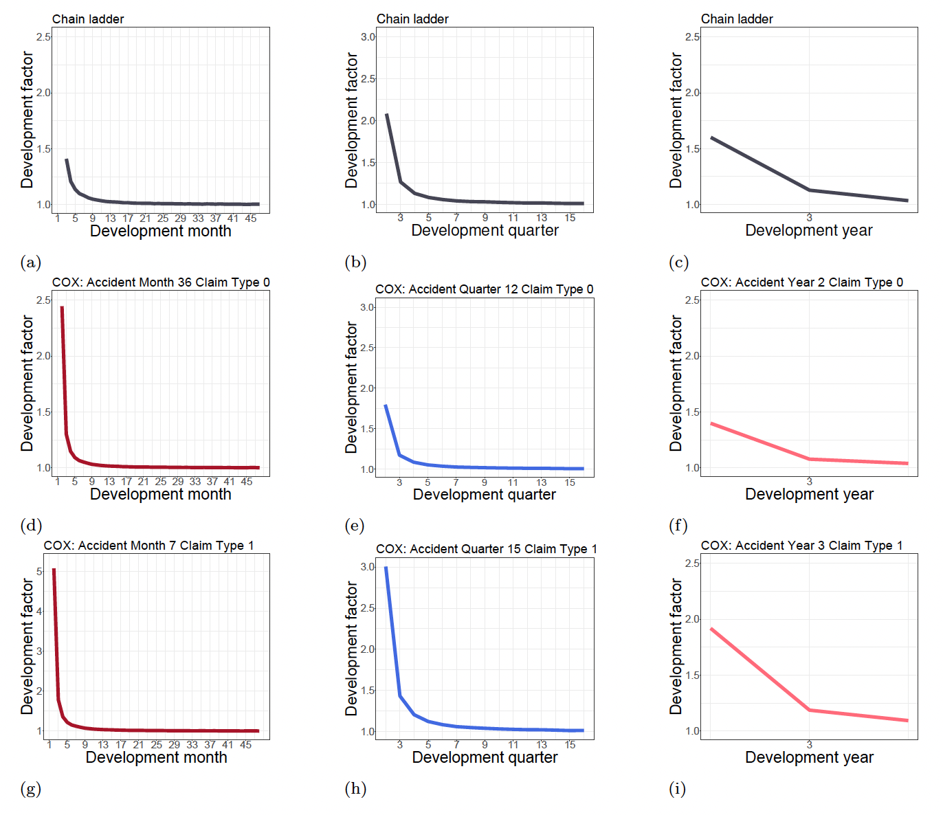
Using our approach we can produce, for each combination of features, the feature-dependent development factors in equation 8. In Figure 3 we produce an example for the COX output illustrated in this Section and compare it with the chain-ladder model. We show for monthly, quarterly and yearly data the development factors fitted with the COX model for some combinations of features (rows two and three). As compared to the chain-ladder development factors (row one), we can capture data heterogeneity by feature.

The feature-dependent development factors in Figure 3 can be plotted with the plot method. For example, in Figure 3b we show the output for AP_o 15 and claim_type 1. As described in Section 2.3, we used AP and claim_type as features.

As we will see below, we need to select the output group code and use it as group_code parameter of the plot method. The output group_code can be found in the group_o column of the long_triangle_format_out$output_granularity output of the predict.ReSurv method. Similarly, the input group_code would be in the group_i column of the long_triangle_format_out$input_granularity output of the predict.ReSurv method.

>>> plot(resurv_fit_predict_q,
         granularity = "output",
         title_par = "COX: Accident Quarter 15 Claim Type 1",
         group_code = 30)

The other main parameters include the granularity of the development factors (either "input" for the input_time_granularity or "output" for the output_time_granularity).

The code for the other feature combinations in can be found in Appendix B.

Figure 3.The first column, shows monthly development factors for the chain-ladder (top panel) and the COX model for the feature combinations Accident Month 36 and Claim_type 0 (center panel) and Accident Month 7 and Claim_type 1 (bottom panel). The second column shows quarterly development factors for the chain-ladder (top panel) and the COX model for feature combinations Accident Quarter 12 and Claim_type 0 (center panel) and Accident Quarter 15 and Claim_type 1 (bottom panel). The third column shows yearly development factors for the chain-ladder (top panel) and the COX model for the feature combinations Accident Year 2 and Claim_type 0 (center panel), and Accident Year 3 and Claim_type 1 (bottom panel).

3. Data application

In this Section, we show a small data application that compares our fitted models on the data from Section 2.2.1 using three different performance metrics defined below. The code is shown for the COX model, but similar computations can be performed with XGB and NN. The three metrics are the Total Absolute Relative Error ($\texttt{ARE}^{\texttt{TOT}}$), Calendar Absolute Relative Error ($\texttt{ARE}^{\texttt{CAL}}$) and the Continuously Ranked Probability Score (CRPS; Gneiting et al. 2004). While the code for the first two metrics is computed in Appendix C, we show here the usage of the built-in function survival_crps for the computation of the CRPS of ReSurv models.

Total Absolute Relative Error $\texttt{ARE}^{\texttt{TOT}}$

We first evaluate the Total (relative) Absolute Errors $\texttt{ARE}^{\texttt{TOT}}$ on the input grid. The $\texttt{ARE}^{\texttt{TOT}}$ is defined as

$$\texttt{ARE}^{\texttt{TOT}} = \frac{\sum_{j,k:k+j>m} |\sum_x O_{k,j}(x)- \sum_x \hat O_{k,j}(x)|}{\sum_{j,k:k+j>m} \sum_x O_{k,j}(x)}, \tag{9}$$

where $\hat O_{k,j}(x)$ denotes the estimated claim counts in accident date $k$ and reporting delay $j$ with features $x$.

The $\texttt{ARE}^{\texttt{TOT}}$ computation for the COX fit is displayed in Appendix C.

Calendar Absolute Relative Error $\texttt{ARE}^{\texttt{CAL}}$

We then want to evaluate our models’ performance a second time diagonal-wise with a different performance metric. We consider the new information available at the end of each calendar date until the end of the duration for which we have data. We call this metric the Total (relative) Absolute Errors by Calendar time ($\texttt{ARE}^{\texttt{CAL}}$). The $\texttt{ARE}^{\texttt{CAL}}$ is defined as

$$\small{ \texttt{ARE}^{\texttt{CAL}}=\frac{\sum^{2m-1}_{\tau=m+1} \sum_{j,k:k+j=\tau }| \sum_x O_{k,j}(x)- \sum_x \hat f_{k,j}(x) O_{k,j-1}(x)|}{\sum_{j,k:k+j>m} \sum_x O_{k,j}(x)}. \tag{10}}$$

The computation of the quarterly $\texttt{ARE}^{\texttt{CAL}}$ for the COX model is shown in Appendix C.

Continuously Ranked Probability Score (CRPS)

The Continuously Ranked Probability Score (CRPS) is defined in Gneiting and Raftery (2007) as

$$\begin{aligned} \operatorname{CRPS}(\hat{S}(\cdot|{x}) ,y) &= \int_{0}^{\infty} \operatorname{PS}(\hat{S}(z|{x}), \mathbb{I}\{y > z\}) \mathrm{d} z \\ &= \int_{0}^{\infty} (\hat{S}(z|{x}) - \mathbb{I}\{y > z\})^2 \mathrm{d} z \\ &= \int^{y}_0 \left(1-\hat{S}(z|{x})\right)^2 dz + \int^{+\infty}_y \left(\hat{S}(z|{x})\right)^2 dz, \end{aligned}$$

with $\operatorname{PS}(\hat{S}(z|{x}), \mathbb{I}\{y > z\}) = (\hat{S}(z|{x}) - \mathbb{I}\{y > z\})^2$ being the Brier Score (Selten 1998; Gneiting and Raftery 2007). We can use correspondence between survival function and predicted development factors (Hiabu, Hofman, and Pittarello 2023) to estimate

$$\begin{aligned} \hat{S}(j|{x})=\frac{1}{\prod^{j}_{l=1} \hat{f}_{k,l}(x)}, \end{aligned} \tag{11}$$

where $\hat{S}(j|{x})$ is an estimator for the survival function ${S}(j|{x}) = P\left(T_i \geq j | {X_i=x}\right).$ The CRPS can be computed with the built-in method survival_crps

>>> crps <- survival_crps(resurv.fit.cox)

The output of survival_crps is a data.table that contains the CRPS (crps) for each observation (id). For comparison among models, we take the average CRPS on the data.

>>> m_crps <- mean(crps$crps)
>>> m_crps
  366.2639

Models comparison

In scenario Alpha, the chain-ladder was expected to work well as the mix of the two claim types has a stable pattern. The results on one of the Alpha simulations from are shown in Section 2.2.1. We observe that the NN model in bold shows the smallest $\texttt{ARE}^{\texttt{TOT}}$, $\texttt{ARE}^{\texttt{CAL}}$ and smallest average CRPS. We seem to prefer the NN model to COX and XGB according to the metrics defined in this section. However, we observe that NN and XGB can be sensitive to hyperparameter choice, and they require the extensive cross-validation procedure that we illustrated in the previous sections. Our models are also compared with the chain-ladder (column one). While the chain-ladder seems to work well, it is outperformed by the other models.

The use of our more sophisticated methods is driven in more complex scenarios like scenario Delta. In Table 7, we show the results for one of the simulation of Scenario Delta. Scenario Delta was described in detail in Section 2.2.1, and it resembles a real world scenario with seasonal patterns. Here, our models significantly outperform the chain-ladder in terms of $\texttt{ARE}^{\texttt{TOT}}$ and $\texttt{ARE}^{\texttt{CAL}}$. The best the $\texttt{ARE}^{\texttt{TOT}}$ and $\texttt{ARE}^{\texttt{CAL}}$ are obtained with the XGB model, which also shows the best CRPS result. The results in Table 6 and Table 7 are taken from the main manuscript replication material and were derived with the procedure described in this paper.

Further Reading

The interested reader can find additional material and information on ReSurv at our website

https://edhofman.github.io/ReSurv/.

It is possible to track the package development at

https://github.com/edhofman/ReSurv.

The ArXiv version of the main manuscript has archive identifier

arxiv:2312.14549.

An RMarkdown version of the code included in this manuscript can be downloaded at

https://github.com/edhofman/ReSurv/blob/main/vignettes/cas_call.Rmd.

The code is also available in the html knitted version at articles/cas_call.html.

Acknowledgments

This project was carried out in collaboration with the Casualty Actuarial Society (CAS) and the CAS Reserves Working Group. We are especially grateful to Mike Larsen, Anton Zalesky and Rajesh Sahasrabuddhe for their valuable comments, which contributed to improvements in both the paper and the software, as well as for their thorough review of our manuscript.